RDP 8710: Transmission of External Shocks in the RBII Model 3. Simulation Properties
November 1987
- Download the Paper 753KB
A full specification of the simulation model is presented in Appendix 1. As was discussed in the previous section, the simulation properties of the model depend on the policy reaction function which specifies the way in which open market operations influence the supply of cash. The level of these operations may depend on a variety of key variables. For the purpose of illustrating the properties of the model, two extreme cases are considered. In the first case, market operations are assumed to react so as to hold the money supply unchanged in response to shocks (referred to as the “money rule”); in the second case, it is the exchange rate which is held (the “exchange rate rule”). A third case, in which the reaction function is specified In terms of several indicator variables (the “multi-variable rule”), is also reported. The exact specification of the reaction functions is shown in Appendix 1.
The properties of the model are examined by analysing responses to three exogenous shocks:
- a permanent non-accommodated fiscal shock, equivalent to 1 per cent of initial GDP;
- a temporary 3 per cent increase in world interest rates, lasting for six quarters;
- a permanent 5 per cent decline in the terms of trade.
Simulations are reported for a period of 40 quarters over the forecast period. Results are reported in terms of deviation from baseline.
The above simulations are performed using the version of the model in which there are no policy reactions to the accumulation of government debt. Debt accumulation effects are considered separately in a fourth simulation which shows the effect of the fiscal shock when debt is fully endogenous and a long-run tax financing mechanism is in operation.
(a) A permanent non-accommodated fiscal exnansion
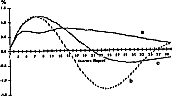
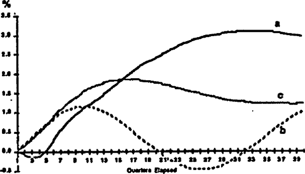
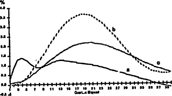
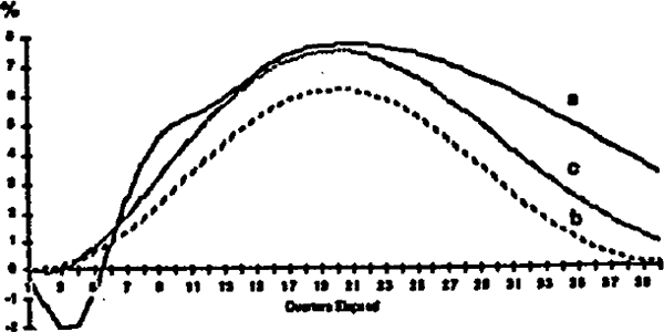
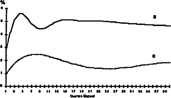
Simulated responses to a non-accommodated fiscal shock are shown in figures 1–5. The case where the money stock forms the objective of open market operations is discussed first. Output increases, with the multiplier peaking initially at 5 quarters and dying out very slowly thereafter. Crowding out is caused by the rise in interest rates, and through direct supply-side effects on investment. The peak multiplier of about 0.7 is a little lower than in earlier versions of RBII, due to the rapid interest rate and exchange rate responses which are now present.
Short-term interest rates respond immediately to the fiscal shock, rising by about 1 per cent in the first yean long rates respond more slowly. Associated with the rise in short-term interest rates is an appreciation of the exchange rate caused by the influence of interest rates on the capital account; the exchange rate movement contributes to crowding out through its effect on net exports. The appreciation is short-lived, however, and gives way after the first year to a depreciation of the exchange rate as the current account moves into deficit, driven by aggregate demand. Over the medium terra, there is a real depreciation, although this moderates towards the end of the period as output declines towards baseline and the current account improves. Consumer prices move with the exchange rate, falling initially due to the appreciation and rising thereafter. Longer simulations confirm that all variables eventually return to baseline.
A Permenent Non-Aecommodated Fiscal Shock

a. money rule;
b. exchange rate rule;
c. multivariable rule.
When the exchange rate rule is followed, the model produces much bigger swings in output. Looser monetary conditions prevail initially, so that interest rates increase only marginally and the exchange rate does not appreciate. This reduces the decline in investment over the first two years and increases the size of the fiscal multiplier under this regime to over one. After about two years, higher domestic demand begins to put downward pressure on the current account and on the exchange rate. To maintain the exchange rate, interest rates continue to increase, peaking after 18 quarters at roughly 3.5 per cent above baseline. This magnifies the crowding out effect and output falls below baseline after fifteen quarters. The contraction arising from these effects turns out to be larger in magnitude than the initial expansion.
As might be expected, the third case, in which market operations are specified as a function of several variables, produces an outcome somewhere between the two extremes. The policy rule is equivalent to a partial accommodation of the fiscal shock in the early stages, slowing the rise in interest rates and tending to increase the immediate expansionary effects on output and prices. After about three years, the tendency for the exchange rate to depreciate implies a tightening of monetary conditions and rising interest rates. By allowing some of the burden of adjustment to fall on the exchange rate, this policy rule moderates the swings in output that would occur under the exchange rate policy rule.
(b) A temporary rise in world interest rates
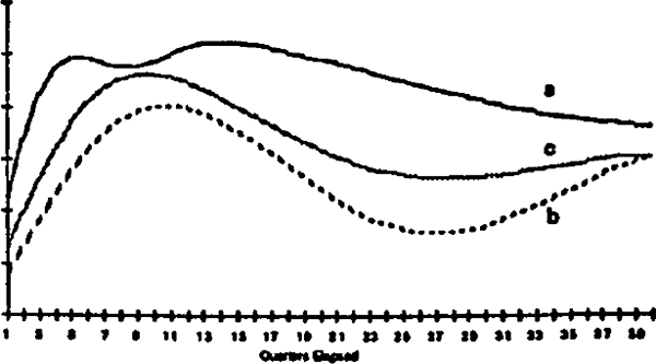
Responses to a temporary rise in world interest rates are graphed in figures 6–10. The rise in world interest rates has two immediate effects: it increases debt servicing costs, thereby adding to the current account deficit) and it induces a portfolio shift into foreign-denominated assets.
The domestic interest rate responses depend upon the policy rule which is being used. Interest rates rise least under the monetary rule, and most under the exchange rate rule. In the latter case, the rise in short-term domestic interest rates must be immediate, and must be greater than the rise in overseas rates in order to maintain portfolio balance with an unchanged exchange rate. The shock is therefore highly contractionary in the short to medium term, with both consumption and investment being crowded out due to higher interest rates. Under the monetary rule, on the other hand, there is a short-run expansion of output because the main burden of adjustment to the change in external conditions is placed on the exchange rate. The depreciation leads to a strong demand stimulus through net exports.
A Temporary Shock to World Interest Rates
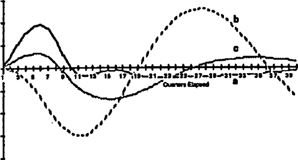
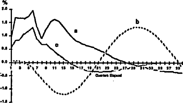
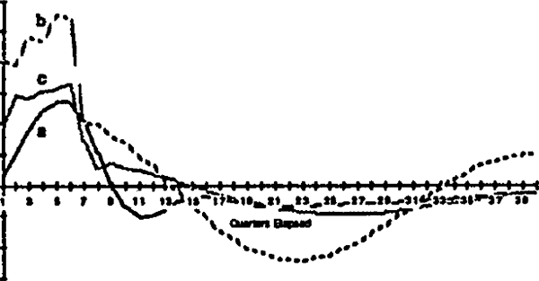
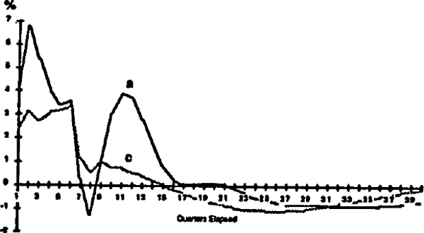
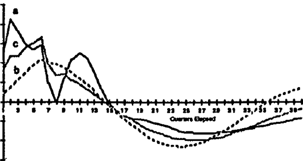
a. money rule;
b. exchange rate rule;
c. multivariable rule.
Results for all three policy rules show a sizeable build up of net external debt in the early stages. This is due to the effect of world interest rates on debt service costs. When the exchange rate is allowed to depreciate, there is a reinforcing valuation effect on the debt.
(c) A permanent decline in the terms of trade
Simulation results for a 5 per cent decline in the terms of trade are shown in figures 11–15. The effects of the shock are clearly contractionary for each of the cases we consider. There are three channels through which these effects operate. Most important is probably the net export channel. This is particularly powerful for the case when the exchange rate rule is in force, since the necessary relative price adjustments are slow to operate and a substantial initial fall in export volumes occurs. Under the monetary rule, on the other hand, the exchange rate depreciates quickly to around its new long run equilibrium, about 5 per cent lower than baseline. This tends to halt the decline in exports much more quickly.
The other main channels through which terms of trade effects operate are through consumption and investment. Both are reduced in response to the shock because disposable income and profitability are each measured in “terms of trade adjusted” units.
With the price level about 2 per cent higher, and the nominal exchange rate about 5 per cent lower, the results appear to indicate that a real depreciation of about 3 per cent is consistent with the new long run equilibrium in the model; this is suggested by the apparent convergence under the monetary rule to a real depreciation of around that magnitude. Under the exchange rate rule, substantial cyclical behaviour is still evident at the end of the ten year period; this policy rule tends to force adjustment onto quantities rather than prices, thus slowing the convergence to long run equilibrium.
A Permanent Decline in the Terms of Trade
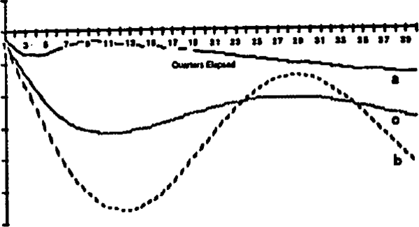
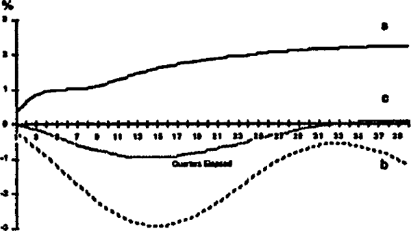
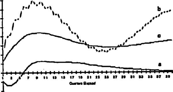
a. money rule;
b. exchange rate rule;
c. multivariable rule.
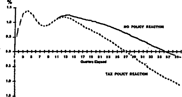
A Fiscal Shock with Endogenous Public Debt
Money rule

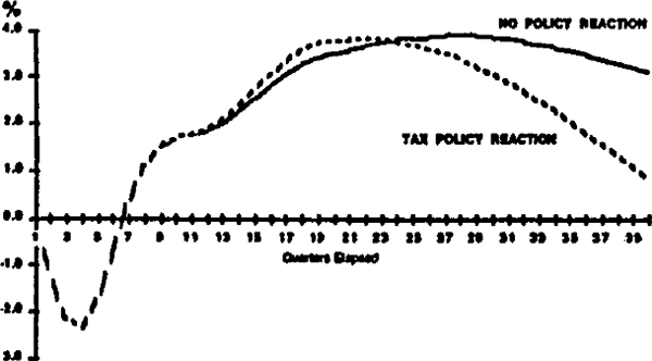
Multivariable rule

(d) An endogenous policy response to government debt accumulation
In this section we reconsider the transmission of a fiscal shock when government debt is fully endogenous. As was pointed out in section 2, this implies the necessity of specifying an additional policy rule which effectively controls the growth of debt. Three alternative mechanisms of debt control were suggested, for the purposes of this section, we assume the endogenous tax rate mechanism operates. This means that the income tax rate is raised, with a lag, in response to a long run increase in the public debt to GDP ratio, thus allowing the ratio to be stabilised. He assume a two year lag in the policy response.
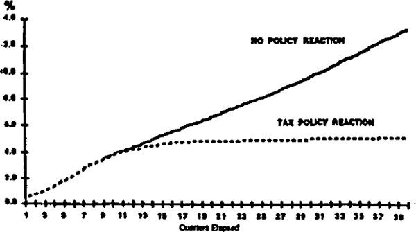
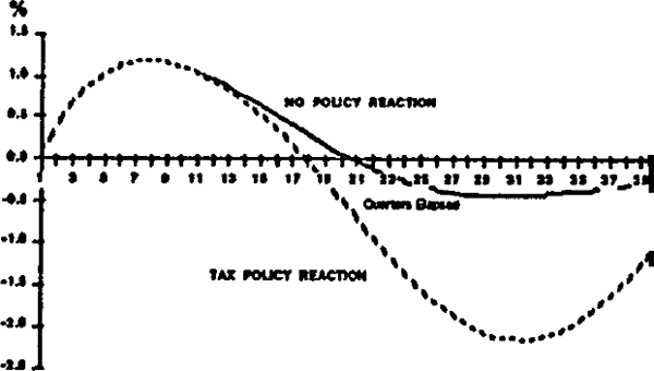
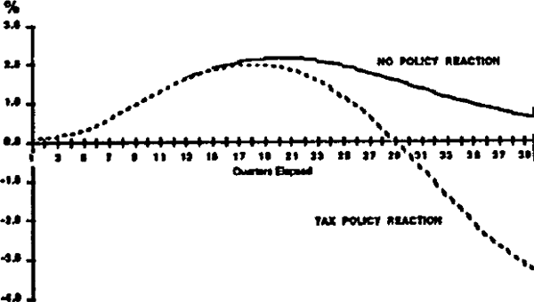
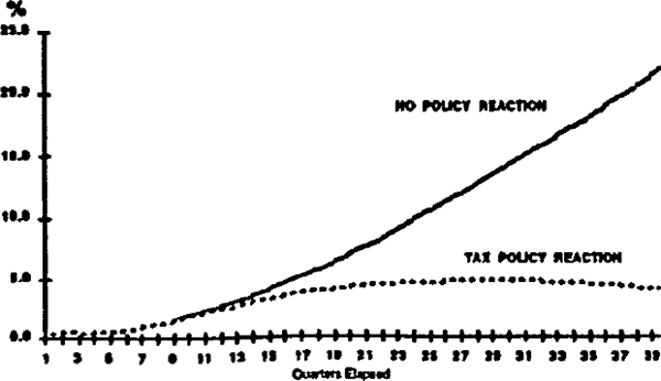
Simulations are conducted under two alternative assumptions about monetary policy: in figures 16–19, a monetary rule is assumed, and in figures 20–23 a multivariate rule for market operations is assumed. Each graph shows responses to the fiscal shock with and without the assumption of tax adjustments to control the growth of debt.
The results show fiscal expansion to be a much less attractive policy than it had appeared when debt accumulation effects were not taken into account. With no tax adjustment, the debt to GDP ratio rises by around 6 percentage points over the 10 year period in response to the shock, and follows a divergent trend. When endogenous tax adjustments are introduced, the average income tax rate rises by about two percentage points after three years, allowing the debt to GDP ratio to be stabilised about two percentage points above baseline. The increase in the tax rate is sustained throughout the simulation period. Under the assumption that the debt to GDP ratio is stabilised at an increased level, a permanent increase in the tax rate is needed to meet the higher debt service costs. This of course is purely illustrative, and assumes that the government sector makes no adjustments on the spending side and that no change in the steady state inflation rate occurs.
The increase in taxation has conventional contractionary effects, causing a downturn in output during the second half of the simulation period that is larger in absolute size than the initial expansion arising from the fiscal stimulus.