RDP 8905: Monetary Policy Instruments: A Theoretical Analysis 3. Choosing an Optimal Policy Rule

The model introduced in the previous section is characterised by an extreme version of nominal neutrality. Output is fixed at the natural rate, and the only possible objective for monetary policy is to stabilise prices. Moreover, it is easy to see that given full information on the part of the policy setter, the optimal policy achieves perfect stabilisation, since it is always possible to devise a rule which exactly offsets the exogenous shocks to the system. The optimal money supply rule, for example, is given by

which, by substitution into the general solution equation (3), can be seen to yield a perfectly stable price level.

The more interesting situation arises when policy is assumed to be set on the basis of less than perfect information. To illustrate this it is assumed that m_t and R_t are observed precisely by the policy setter, but prices are observed with error at the time instruments are set. This has the effect that neither of the random disturbances can be observed contemporaneously. The specific assumption is that a signal is observed, where

and w_t is an independent disturbance with zero mean. The policy instrument is then specified as a linear function of observable variables. Thus

or equivalently

where

depending on whether policy is thought of as controlling the interest rate or the money stock. A pure interest rate rule (one that is not expressible as an inverted money rule) arises in the case where ρ₁ is zero.

Substituting the policy rule (5) into the general solution equation (3) yields the following solution for the price level in terms of the exogenous variables:

so that the variance of p_t is given by

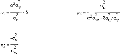
It is assumed that the objective of policy is to minimise this variance, and it can be shown after some fairly straightforward algebra that the optimal choice of weights is given by

What is the intuitive interpretation of these results? If one interprets the system as describing the operation of a money rule (as in equation (5)), then π₁ and π₂ represent the respective weights given to the interest rate and the price level signal in monetary responses. The weight given to interest rate smoothing, rises with the relative variance of monetary shocks to real shocks. This is almost exactly the conclusion obtained by Poole in his one-period framework. The optimal size of response to the price level signal depends on the signal's accuracy. As the accuracy increases ( approaching zero), the optimal policy becomes progressively more activist in responding to the signal (π₂ increasing).

An alternative way of interpreting the solution is in terms of an interest rate rule, as in equation (6). The parameters ρ₁ and ρ₂ then represent weights given to the money supply and the price signal in the policy response function. Money is given a high weight when the money demand function is very stable ( approaching zero); conversely, its weight is zero in the case of extreme instability ( infinite). In this case, the money demand function is so unstable that information about money carries no information about prices, and the optimal policy responds only to the (imperfect) price signal. This may be taken as a limiting case. Although the ultimate objective of policy has nothing to do with the money supply, in general it is optimal for an interest rate policy rule to respond to money because the money stock contains information which can be used to improve the estimate of the price level. Only in the extreme cases where money demand disturbances have infinite variance, or the price level signal is perfectly accurate, is money given no weight at all in the optimal policy rule.