RDP 8910: An Analysis of the Determinants of Imports 6. Results
December 1989
- Download the Paper 967KB
Properties of the Time Series
Eight time series were used in the estimation procedure:
| M: | real total merchandise imports |
| EM: | real endogenous imports |
| Y: | real GDP |
| D: | real GNE |
| RPM: | ratio of the total imports deflator to the GDP deflator |
| RPEM: | ratio of the endogenous imports deflator to the GDP deflator |
| RPX: | ratio of the merchandise exports deflator to the GDP deflator |
| OT: | hours of overtime per employee |
The natural logarithm of each series was used throughout the estimation. The base year for all price indices and real variables was 1984/85. All estimation was carried out using quarterly seasonally adjusted data over the period from September 1974 to September 1989.[11] (See Appendix 1 for further details.)
The results of the stationarity tests can be found in Appendix 2. For both total and endogenous imports, and GNE, these tests indicate clear evidence of one unit root at a 1 per cent significance level. GDP also appears to have a single unit root, although this could only be accepted at a 5 per cent level of significance. There is also evidence of a time trend in all of these variables.
The results for the relative price terms and overtime are less conclusive. There is evidence supporting the existence of both one and two unit roots. To an extent this ambiguity may be due to the relatively short estimation period used, as the statistical tests need long runs of data to differentiate between alternative models of the time series. Accordingly, these series were examined over a longer time period using the NIF data base for earlier periods; we found convincing support for the existence of one unit root. (These results are available on request from the authors.)
Long Run Regression Results
The cointegrating relationships between imports and its explanators are estimated over the period from September 1974 to September 1989, and the results can be found in Table 1. At a 5 per cent significance level, −3.17 is the critical value for the ADF test, and at the 1 per cent level it is −3.77.[12] These results suggest that four cointegrative relationships have been identified.
Overtime is not included in any of the long run relationships, as it is not necessary for cointegration. This result is consistent with our model, as we include the overtime variable to capture short term cyclical demand effects, specifically, to identify times of demand spillover into imports.
The coefficients on each of the explanators in Table 1 can be interpreted as being estimates of the long run import demand elasticities of the respective explanators. Three important points emerge from an examination of this Table. First, all coefficients have the expected sign. Secondly, the demand elasticity appears to be insensitive to the choice of GNE or GDP as the activity explanator: it is around 1.9 for both endogenous and total imports. Thirdly, the choice of activity variable affects the import price elasticity. Using GDP as the demand explanator results in a price elasticity of 0.6 for total imports and 0.8 for endogenous imports. Alternatively using GNE as the demand explanator results in lower price elasticities of 0.4 and 0.5 for total and endogenous imports respectively.
We are not able to tell whether the relative price of exports is a significant explanator, because the standard errors have an unknown distribution. The inclusion of RPXt increases the ADF statistic for total imports, and hence our level of confidence that a cointegrating relationship exists. By contrast, the inclusion of RPXt reduces the ADF statistic for endogenous imports. Nevertheless, in both cases, cointegrative relationships are found with RPXt included.
It is worth briefly comparing these results with the results of other studies. Macfarlane (1979) compares elasticity estimates from a number of Australian import demand models which are estimated over the 1960s and early 1970s. Broadly the income elasticity estimates are lower than ours, ranging from 0.7 to 1.2, although in 3 of the 11 studies cited the income elasticity is constrained to 1. On the other hand, the significant relative price elasticities tend to be higher than our estimates, ranging from −0.5 to −1.6, although in 3 studies they are insignificant. These differences may reflect structural changes in the Australian economy or, alternatively, they may reflect differences in estimation techniques.
Our results can also be compared with estimates from other countries. Krugman (1988) estimates price and income elasticities for a number of countries between 1971 and 1986. Some of his income and relative price elasticities are, respectively: Canada 1.66 and −1.45, Germany 2.83 and −0.09, the US 1.31 and −0.93, Japan 0.8 and −0.42, Italy 1.31 and −0.68, Belgium 1.99 and −0.25, and the Netherlands 2.66 and −0.22.[13] Our income and price elasticities are clearly well within this range.
Error Correction Model Results
For each of the four cointegrated relationships discussed above, an error correction model is formed. This involves regressing the change in imports on the residual from the cointegration regression, one period lagged, and four lags of changes in imports, demand, relative prices and overtime. In order to improve the accuracy of the significant coefficient estimates, those variables whose coefficients were statistically insignificant were excluded from the regression. The results of these regressions can be found in Appendix 3.
In the following discussion, we concentrate on Models 1 and 2. These are the total and endogenous imports equations which use GDP as the demand explanator.
Some interesting observations can be made about these models. For both models the cointegrating term is statistically significant. In fact, around 70 per cent of the equilibrium error in the previous period feeds through into current period changes in imports. Changes in the relative prices both of imports and exports also significantly affect the short run dynamics of the system. And the overtime variables, although not individually significant, have the expected sign. For each model the null hypothesis of both overtime coefficients being zero is rejected at a 5 per cent level of significance.
The explanatory power of these error correction models is relatively high at around 60 per cent. The inclusion of both the relative price of exports and overtime as explanators increases the explanatory power by some 15 per cent.
Table 2 presents the impact demand and price elasticities which have been calculated from the reduced form of the error correction models.[14] From this Table it is interesting to note that while most of the impact of a change in demand occurs in the first 2 quarters, price effects have an impact over a much longer period.
| LAGS | 1 | 2 | 3 | 4 | 5 | 6 | 7 | 8 |
|---|---|---|---|---|---|---|---|---|
| MODEL 1 – Total Imports | ||||||||
| Demand | 1.41 | 0.34 | 0.08 | 0.02 | 0.01 | 0.00 | 0.00 | 0.00 |
| Price-Imports | −0.07 | −0.43 | −0.51 | −0.24 | 0.46 | 0.11 | 0.03 | 0.01 |
| Price-Exports | −0.25 | 0.00 | 0.56 | 0.51 | −0.26 | −0.06 | −0.02 | 0.00 |
| MODEL 2 – Endogenous Imports | ||||||||
| Demand | 2.14 | −0.15 | −0.05 | −0.02 | −0.46 | 0.34 | 0.09 | 0.02 |
| Price-Imports | −0.53 | −0.18 | −0.06 | −0.41 | 0.37 | 0.05 | −0.01 | 0.07 |
| Price-Exports | 0.27 | −0.29 | 0.28 | 0.51 | −0.30 | 0.02 | −0.12 | −0.09 |
The short run demand elasticities of the two models are quite different. In Model 1, the initial impact of a 1 per cent change in demand is a 1.4 per cent change in imports, and over the following quarters there are positive impacts which sum to the long run 1.9 per cent change. In the Model 2, however, ‘overshooting’ is evident. In the first period after a 1 per cent change in demand, the impact on imports is 2.1 per cent, and then this is partially reversed. These quite different paths to the new equilibrium in response to a demand shock can be explained by there being significant lagged changes in demand and imports in the ECM for Model 2, whereas there were none for Model 1.
The impact price elasticities are more variable over time much of which does not seem credible. However, the general trends which can be drawn from the table are that changes in the relative price of imports tend to have a negative impact on import demand in the first four quarters but they ‘overshoot’, and hence there is some correction in the following four quarters. Changes in the relative price of exports tend to have a positive impact on imports in the first four quarters but they too ‘overshoot’, and there is some correction in the following four quarters.
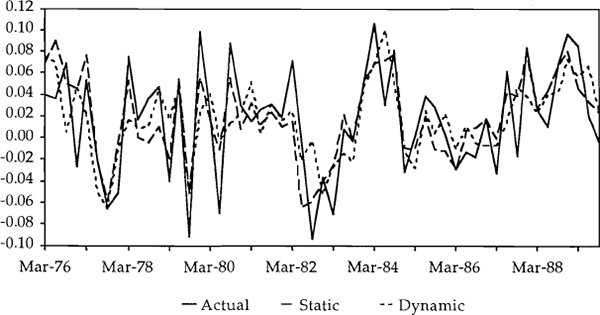
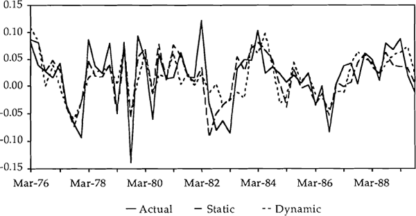
In Charts 3 and 5 the actual and fitted changes in the log of imports have been plotted for Models 1 and 2 respectively. Each chart shows changes in the actual series and two fitted series. The first of the fitted series is a static simulation – i.e. lags of actual imports are fed through the model – while the second shows a dynamic simulation – i.e. lags of the generated imports series are fed through the model.
MODEL 1 SIMULATION
MODEL 1 SIMULATION
MODEL 2 SIMULATION
MODEL 2 SIMULATION
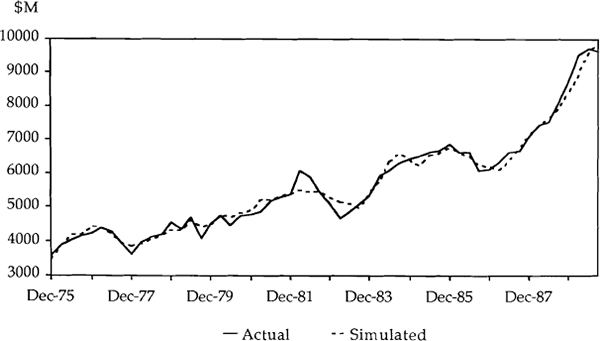
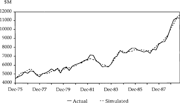
In Charts 4 and 6, the changes in imports are converted into levels – only the dynamic simulation is shown.
From these charts it is interesting to note how well both simulated series track the actual series. For both models the large movements in imports in the early 1980s were not well tracked. However, in the most recent surge in imports, although the models have underpredicted the total growth, they have picked up a significant amount of the growth – even when using a dynamic simulation. Between September 1986 and June 1989 total imports increased by 52 per cent while Model 1 predicted (dynamically) growth of 47 per cent. Over this same period endogenous imports increased by 60 per cent while Model 2 predicted (dynamically) growth in imports of 55 per cent.
As Table 3 shows, in this recent period all of the explanators of import growth, other than the relative price of exports, moved in a direction to encourage growth in imports. Most dramatic were the falls in the relative prices of imports and the growth in activity.
| Total Imports | 51.7 |
|---|---|
| Endogenous Imports | 59.9 |
| GNE | 17.6 |
| GDP | 12.2 |
| Relative price of total imports | −26.9 |
| Relative price of endogenous imports | −25.2 |
| Relative price of exports | −2.1 |
| Overtime | 21.5 |
An interesting question is which of these explanators made the largest contribution to this growth in imports? In Table 4 we use our models to dynamically simulate growth in imports while controlling for growth in the alternative explanators. Taking each explanator in turn, we impose no change in that explanator from September 1986 onwards, and then simulate our models to determine the level of import growth predicted. The difference between these predictions and the import growth predictions when all variables are changing, determine the percentage points of growth contributed by each explanator (as quoted in Table 4). Because our model is non-linear in levels, the sum of the individual contributions is not equal to the total amount of growth predicted by the respective models.
| Model 1 | Model 2 | |
|---|---|---|
| Total growth predicted | 47.4 | 54.7 |
| Percentage points of import growth contributed by: | ||
| Growth in GDP | 24.9 | 28.3 |
| Falls in the relative price of imports | 31.1 | 37.1 |
| Falls in the relative price of exports | −2.9 | −2.2 |
| Growth in overtime | 0.4 | 0.2 |
For both models a larger contribution to growth in imports was made by falls in the relative price of imports than by growth in activity. These two variables were the most significant contributors. The negative contribution of the relative price of exports was small because of its relative lack of movement.[15] Although overtime grew significantly over the period its contribution was also small. This is a consequence of the form of the models. First, because overtime is not included in the long run equations, it cannot have a long lasting impact on import demand. Secondly, our equations are estimated with all variables in logarithmic form. Because the coefficient on demand in the long run equation is greater than one, imports respond more than proportionately to surges in the level of demand. To an extent this reduces the need for a variable such as overtime and thus reduces its coefficient estimates.
Out of Sample Tracking Performance
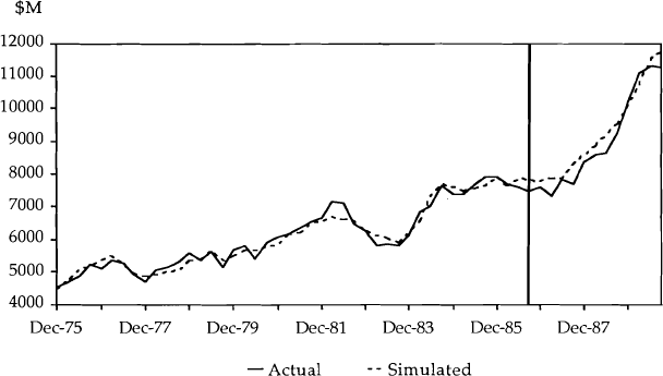
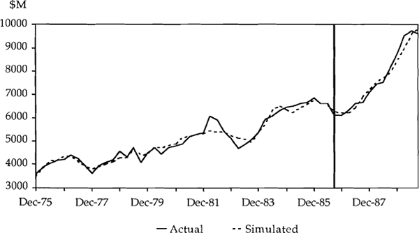
There is valid concern that the performance of our models over the most recent period reflects primarily the fact that the models have been estimated over this period. To test the out of sample stability of our models we re-estimated both equations in their preferred forms (i.e. with the explanators from Appendix 2), between September 1974 and September 1986. We then simulated, using the new coefficient estimates, over the period from September 1986 to September 1989.
Charts 7 and 8 show the simulations for the total and endogenous import models respectively. These charts suggest there has not been a significant change in the relationship between imports and its explanators over the recent period. Further, they suggest that if, in September 1986, we had accurate forecasts of activity, overtime and price profiles for the next twelve quarters, the rise in imports could have been accurately predicted.
MODEL 1 SIMULATION
MODEL 2 SIMULATION
A post-sample predictive test developed by Davidson et. al. (1978) is used to test more formally
the out of sample tracking performance of our models. This consists of estimating the model up
to some date T, which we have taken to be September 1986, and then using the model to simulate
for  periods
past T, in our case up to September 1989. Davidson et. al. (1978) developed a test statistic
which tests whether the forecast residuals differ significantly from the residuals within
sample. This test is based on the sum of squared residuals.[16]
The results of our tests, reported in Table 5, lead us to convincingly accept the null hypotheses of stability in the coefficient estimates, confirming our conclusions from Charts 7 and 8.
| Equation | Test Statistic | Critical Value | |
|---|---|---|---|
| 1% | 5% | ||
| Model 1 – Static | 12.86 | 26.22 | 23.34 |
| Model 1 – Dynamic | 9.87 | 26.22 | 23.34 |
| Model 2 – Static | 5.38 | 26.22 | 23.34 |
| Model 2 – Dynamic | 4.25 | 26.22 | 23.34 |
Footnotes
This sample period was chosen because the Australian Bureau of Statistics publishes and revises a consistent constant price series for imports over this period. [11]
See Engle and Granger (1987), Table II, p. 269. [12]
For each country Krugman estimates the model: Mt = αDt + βRPt + λRPt−l. He does not test these series for their order of integration, nor these relationships for cointegration. To calculate his long run price elasticities we have summed the coefficient estimates β and λ. This is only strictly correct if true cointegrative relationships have been identified. [13]
These elasticities must be interpreted with care because the equation that we have estimated actually comes from a system of equations, as described in Section 4. To generate these short-run elasticities one is implicitly assuming that the 1 per cent change in demand (or price) is generated independently from the stochastic term in the imports equations. Although this may be an unrealistic assumption, these short run elasticities are useful for understanding the implied paths of adjustment of the model, which is important if the model is being used for single equation forecasting. [14]
The substantial increase in the foreign currency price of our exports since 1986 was partially offset by the appreciation of the $A, leading to the fall in the relative price of exports to the GDP deflator shown in Table 3. [15]
 , under the null hypothesis of no change
in the parameters β and σ2, the test statistic is:
where
  is the usual estimate of the variance of the error
within the sample:
[16]


