RDP 9001: Is Pitchford Right? Current Account Adjustment, Exchange Rate Dynamics and Macroeconomic Policy 3. The Sticky Real Exchange Rate Model

The model of section 2 assumes that the real exchange rate, and hence the current account, adjust smoothly to all shocks. To what extent are the above results dependent on this assumption ? This is an important question since substantial evidence suggests that real exchange rates do not, in fact, adjust steadily and quickly to eliminate current account imbalances. (See e.g. Dornbusch 1989.)

In this section I relax the market-clearing assumptions of section 2. As it turns out, with one significant exception, the results of that section are essentially unchanged. The exception is that the laissez-faire outcome is now inefficient and so a welfare-enhancing role can be found for government policy.

The market-clearing assumption is relaxed by no longer requiring savings to be equal to desired savings in each period; rather, savings adjusts to desired savings by an error-correction mechanism:

Equation (17) introduces inertia to current account adjustment. Savings in period t is equal to savings in the previous period plus a proportion, γ, of the difference between desired savings in period t and the previous period's savings. Š_t is given by equation (8), above. The source of this inertia is an assumed stickiness in the real exchange rate.^[13] The market-clearing model (S_t = Š_t) is a special case of this model; it occurs when γ = 1.

Making all the appropriate substitutions, the expression for the real exchange rate can be derived: ^[14]

Equation (18) differs from its market-clearing counterpart (11) in that lagged values of q and a are present, along with the parameter γ. Note that (18) collapses to (11) when γ = 1. The asset accumulation equation (7) is unchanged, since it is an accounting identity. The steady state expressions, (12) – (14), are also unchanged, since S = Š in the steady state.

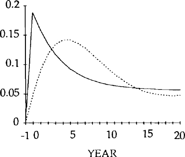
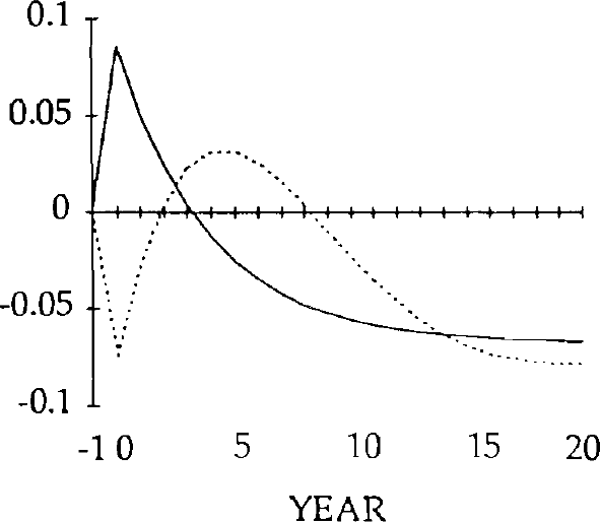
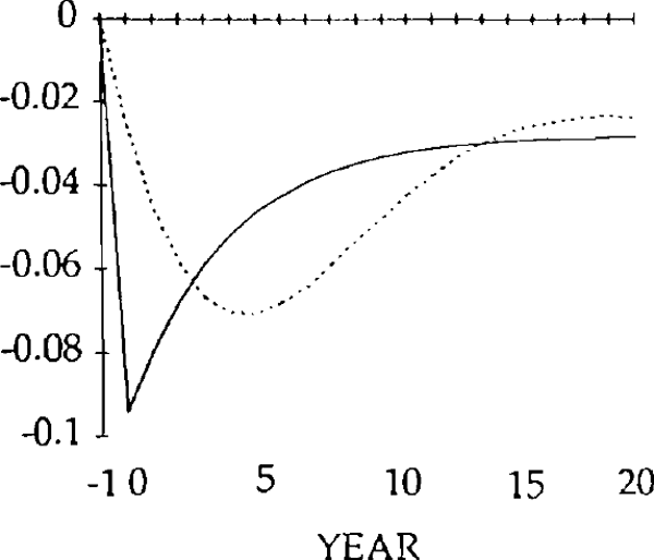
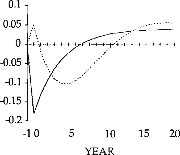
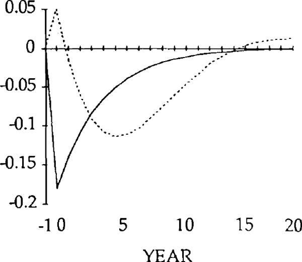
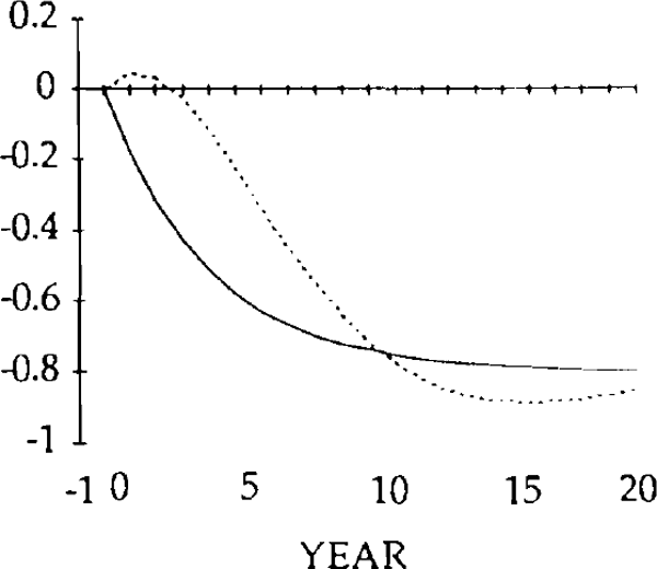
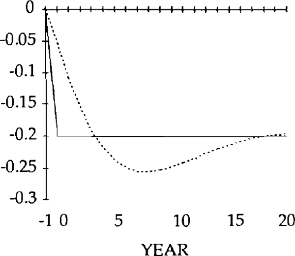
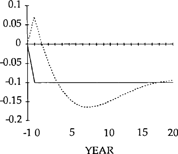
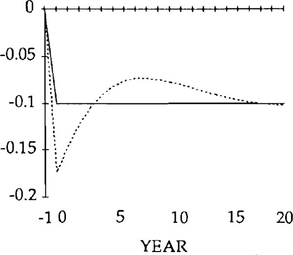
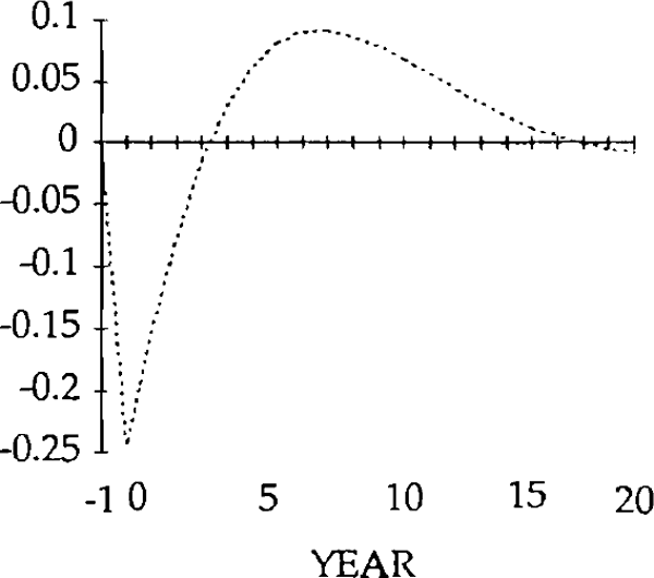
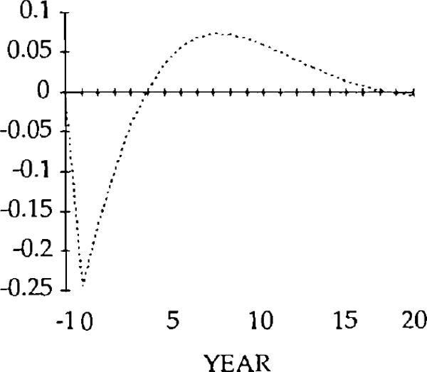
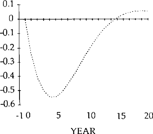
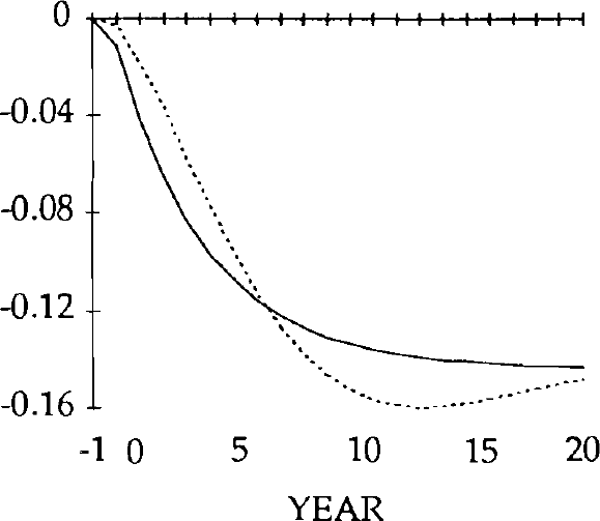
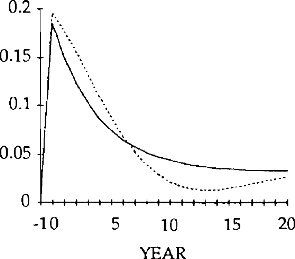
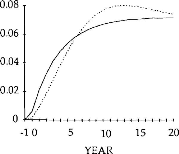
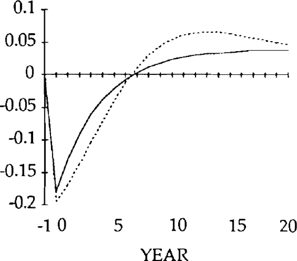
Figures 9 – 26 compare the effects of y shock of −0.20 and x and z shocks of 0.20, for the market-clearing and sticky real exchange rate models. The latter are simulated under the assumption that γ = 0.25, implying that one quarter of disequilibrium savings is eliminated each year.

REAL DOMESTIC EXPENDITURE SHOCK (x)

u = 0.25

— MARKET CLEARING

.... STICKY PRICES (γ= 0.25)

REAL EXPORT SHOCK (y)

u = 0.25

— MARKET CLEARING

.... STICKY PRICES (γ = 0.25)

REAL IMPORT SHOCK (z)

u = 0.25

— MARKET CLEARING

.... STICKY PRICES (γ = 0.25)

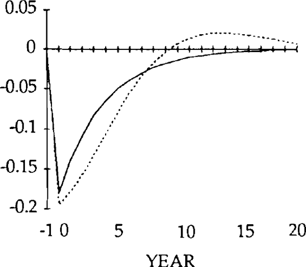
Turning first to the y shock i.e. an exogenous falls in exports, we can see that, unlike the market-clearing case, the trade and current accounts (figures 18 and 19) will be affected when the real exchange rate is slow to adjust (figure 15). The initial fall in exports (figure 17) is almost as large as the exogenous shock; furthermore, imports (figure 16) do not fall sufficiently to offset the fall in exports. In fact they initially increase, for reasons explained below. Consequently, the trade balance becomes negative. ^[15]

Figure 16 shows the effects on real imports of the y shock. Notice that in years 0 and 1, imports actually rise, despite the depreciation of the real exchange rate. Because the real exchange rate is slow to depreciate, the net reduction in exports following the negative shock to y is relatively large. The result is a deficit on the balance of trade. The counterpart to a trade deficit is an excess of domestic spending over domestic production. Part of that excess spending will fall on imports; the net result is an increase in imports in years in 0 and 1.

By year 2, the real depreciation is large enough for imports to have fallen (relative to their initial position). The trade account is still in a deficit position, however, until year 4, when it becomes a surplus. This surplus lasts for several years, and is due to overshooting of the real exchange rate i.e. in years 4 through 17, the value of the real exchange rate falls below its steady state value.

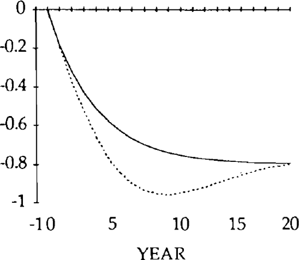
The initial, large, current account deficits lead to the build up of a considerable stock of foreign debt (figure 20). Despite the existence of current account surpluses from year 4, this debt is not eliminated until a further 11 years have elapsed. Eventually, the steady state is reached, characterized by equal reductions in imports and exports, and a trade balance and debt level of zero. However, as figures 15–20 show, stickiness in the real exchange rate can generate long cycles in the trade and current accounts, the real exchange rate, and the stock of net foreign assets.

The effects of the x shocks are shown in figures 9–14. The real exchange rate is slower to rise than in the market-clearing case; it is also slower to fall (figure 9). As a result, it is overvalued (relative to its market-clearing path) from years 3 through 14. Correspondingly, the trade and current account deficits are also larger during that time (figures 12 and 13).

Figure 10 shows that, when the real exchange rate is sluggish, the initial effect of the x shock is to decrease imports. Because of the slow initial rise in the real exchange rate, the crowding out of exports is relatively small (figure 11); consequently, so is the increase in domestic spending on domestic goods. Total domestic expenditure in fact falls relative to production, implying a fall in spending on imports.^[16]

Consistent with this result, the trade balance is in a surplus position, with the fall in imports exceeding the fall in exports. The trade and current account balances become negative in year 1, but for that year and the next the deficits are smaller than for the corresponding years in the market-clearing case. As a result of the initial surplus and the relatively small deficits which follow, the stock of debt takes longer to accumulate when the real exchange rate is sticky than when it is not (figure 14).

The effects of the z shocks are shown in figures 21–26. Qualitatively, the adjustment paths in both of the models are similar. The real exchange rate falls, the current account balance gradually adjusts and the level of debt is eventually eliminated. The quantitative differences are due to the slow response of the real exchange rate, resulting in a slower adjustment process.

The results of this section show that a current account deficit will be self-correcting even if the real exchange rate exhibits some inflexibility. All that is needed to achieve this result is a reasonable institutional assumption, γ ≠ 0 i.e. that the real exchange rate, while sluggish, adjusts eventually to its equilibrium value.

Footnotes

Stickiness in the real exchange rate is an example of a real rigidity which can occur due to a variety of imperfections in product and labour markets. These imperfections need not be due to institutionalized rigidities and may reflect more subtle influences, e.g. asymmetries in the information available to participants in a bargaining process. See Blanchard and Fischer (1989), Ch 9, for an analysis of the sources and effects of real rigidities. [13]

Note that the market-clearing condition d + d^* = 0 is retained in deriving equation (18). This is consistent with a sticky real exchange rate model provided that d is now interpreted as the effective domestic excess demand for domestic goods. The market for domestic goods will therefore still “clear”, but only in the sense that purchases are identically equal to sales. See Benassy (1982) for an analysis of models of this type. [14]

Recall that, when the real exchange rate is sticky, realized and desired savings are no longer equal, except in the steady state. Desired savings are unaffected by the y shock, but given the above inequality, realized savings are changed by the shock to export demand; thus, so is the current account. [15]

This result is not a necessary consequence of the sticky real exchange rate assumption. For a sufficiently large value of σ (so that nearly all excess domestic spending falls on domestic goods) imports will rise (due to the real appreciation) and a trade deficit will result, just as in the market-clearing case. [16]