RDP 9004: Saving and Investment in the 1980s 3. Influences on Private Saving
August 1990
- Download the Paper 2.8MB
3.1 Consumption Smoothing
The idea that households use savings to smooth their consumption patterns over lime forms an important unifying principle in the literature on saving behaviour. Friedman's early formulation of this idea took the pragmatic approach of assuming that households consume a proportion of their permanent incomes, while avoiding placing tight theoretical restrictions on the way permanent and current incomes are related. This relationship was to be determined empirically, which was typically done by assuming permanent income, and hence consumption, are related to current income according to some distributed lag. It was then thought that additional variables such as interest rates or demographic variables could be included and the estimated parameters could be used for forecasting and policy analysis. In reviewing the performance of such models in Australia, Williams (1979) concluded that their record was poor. For forecasting purposes, they were often outperformed by simple extrapolations, and they generally underpredicted levels of household saving in the 1970s.
While poor empirical performance may have been one reason for a change of approach, a more powerful one was probably the influential critique made by Lucas (1976), who questioned the possibility that a structural consumption function existed at all. Interpreting permanent income to encompass expected future income levels, Lucas argued that the relationship between permanent and current income would change as the underlying process generating incomes changed. Thus although there is a structural relationship between consumption and permanent income, standard consumption functions are incorrect to posit a stable relationship between permanent and observed incomes. Lucas made these criticisms from the standpoint of the rational expectations paradigm, but a strict rational expectations assumption is not necessary to the argument: it merely asserts that the effect of a rise in current income on consumption is not mechanical because the response made by households will depend on the way households use information about the extent to which that rise is permanent or temporary.
The effect of the Lucas critique on the study of consumption behaviour was reinforced by the work of Hall (1978), which appeared to offer satisfactory empirical results while also avoiding the basic problem raised by Lucas. Hall's paper, and numerous subsequent studies built on the same approach, aimed to tie the idea of consumption smoothing into an explicit microeconomic framework that has directly testable implications, without having to construct proxies for permanent income. Put in fairly general terms, the approach models consumption as the outcome of a lifetime optimisation problem, in which a representative consumer maximises the expected value of some lifetime utility function subject to a lifetime budget constraint requiring the discounted value of consumption to be no greater than the discounted value of income from all sources. An implication of those assumptions is that the timing of consumption expenditures is independent of the timing of income receipts, and the testing of this implication has been central in the empirical literature.
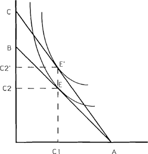
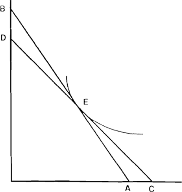
To summarise the main principles of this type of model, Figures 25 to 27 provide a simple two-period representation. The indifference curves represent preferences for current as against future consumption, while the slope of the budget line in each case is given by the real interest rate. The points illustrated are as follows:
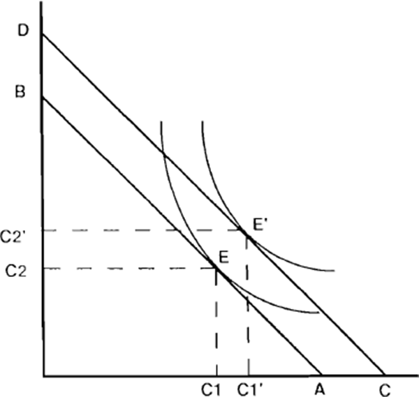
- A temporary increase in current income causes a rise in consumption which is spread between current and future periods (Figure 25). Similarly, an expected increase in future income will affect consumption in both periods.
- A rise in the interest rate, holding initial wealth constant[10], has an ambiguous effect on current consumption because the income and substitution effects are working in opposite directions (Figure 26).
- A rise in the interest rate holding the non-interest income profile constant has an unambiguous negative effect on current consumption, provided the consumption and income profiles are sufficiently similar in the initial equilibrium (Figure 27). In terms of the diagram, point E represents the time profile of non-interest income receipts, and this point must lie on all budget constraints obtained by varying the interest rate, since it is always feasible to consume income as it accrues. If the initial optimum was also at point E, the interest rate change would represent an income-compensated change in relative prices, so that only the substitution effect would operate.[11]
The potential ambiguity of the interest rate effect causes a certain amount of confusion, but in fact a strong case can be made that the substitution effect predominates, making the theoretical effect of a rise in interest rates unambiguously negative. The reason for this is that in aggregate, the private sector receives a very small proportion of its total income in the form of net interest payments. Thus if one follows the approach of modelling aggregate consumption as being determined by a representative consumer, then in terms of the diagrams, that consumer would be in a position much more like Figure 27 than Figure 26. Developing this argument in a multi-period framework, Summers (1981) concluded that for realistic paths of labour income, the income effect of a change in interest rates is very likely to be negligible.
The paradigm of intertemporal optimisation is quite flexible and, with various modifications and extensions, describes a wide range of phenomena.[12] In this sense it is not so much a predictive theory as a modelling strategy. Adherents to the approach argue that it provides a disciplined framework for incorporating whatever additional factors are thought to be important, such as bequest motives, borrowing constraints, or tax distortions; in each case the approach requires that such features be incorporated through modifications to either the utility function or to the set of budget constraints, as opposed to what is seen as the more ad hoc procedure of directly modifying a consumption function. On the other hand, Carroll and Summers (1989) have argued that the representative consumer paradigm is itself ad hoc because of the simplifying assumptions needed to give it observable content, and because there is too much diversity between households to justify representing the aggregate as a single agent.[13] Citing data from the U.S. Consumer Expenditure Survey, they show that most saving is done by a relatively small group of high wealth households which is not large enough to also account for the majority of consumption expenditure; in other words, the bulk of the saving and consuming are being done by different groups. Household Expenditure Survey data in Australia support a similar conclusion.
Empirical implementations of the intertemporal optimising model are typically based on variants of the following equation:
| where | ct represents consumption at t |
| rt is the after tax real interest rate | |
| ut+1 is a forecast error representing revisions to expectations about permanent income. |
Technically this equation can be derived as a first order condition of the consumer's optimisation problem.[14] The intuitive interpretation is that the expected allocation of consumption between the current and future period depends only on the interest rate; when the real interest rate is high, current consumption is reduced relative to consumption in the future, so that expected consumption growth is increased. A testable implication of the theory is that current and lagged variables other than the interest rate do not help to predict future consumption growth, these variables being notionally incorporated in the current estimate of permanent income. This empirical framework has the important advantage that it can be tested without constructing estimates of permanent income itself.
The earliest study along these lines, by Hall (1978), assumed a constant real interest rate and thus focussed mainly on the question of whether or not current income variables entered the equation significantly. Hall's results broadly supported the view that current income effects were not significant, although a current wealth effect could be detected. In a similar study of Australian data, Johnson (1983) found significant effects from current income, although it could still be claimed that consumption was close to a random walk, as Hall had originally predicted. Some of these and other early results were generally obtained by estimating the consumption equation in levels rather than differences, and were thus subject to problems of possible non-stationarity.
Subsequent studies based more closely on equation (1), and with well-defined alternative hypotheses concerning the role of current income, have generally been less favourable to the model. Two results have emerged fairly consistently. The first has been a failure to obtain significant interest elasticities; estimates by Hansen and Singleton (1983) Campbell and Mankiw (1989), Carroll and Summers (1989) and Zeldes (1989) all showed the interest elasticities to be small and insignificant.[15] Hall (1989) concluded that the elasticity of consumption with respect to the interest rate is probably zero, although Mankiw (1985) did find significant elasticities when modelling the durable and non-durable consumption components separately. A second finding that is now well supported in the empirical literature is that current income has a significant, though less than one-for-one, effect on current consumption, in contrast to the basic premise of the intertemporal optimising model. Studies by Flavin (1981), Hayashi (1982) and Campbell and Mankiw (1989) found significant current income effects, as did McKibbin and Richards (1988) in an implementation of Hayashi's approach using Australian data.
The results by Campbell and Mankiw were obtained by the fairly simple approach of augmenting equation (1) to include expected income growth as an additional explanatory variable. This was found to have a coefficient of about 0.5, leading to the interpretation that roughly half of consumption growth is related to income growth, while the remainder is determined consistently with the optimising model. These are close to the proportions estimated by McKibbin and Richards for Australia. Campbell and Mankiw concluded that consumers accounting for half of total consumption face borrowing constraints which lead them to use a rule of thumb matching consumption to current income. This inference was disputed on theoretical grounds by Zeldes (1989), who showed that the effect of borrowing constraints in an optimising framework would be to reduce average levels of consumption in all periods rather than to make consumption follow the path of current income. On this basis, the Campbell and Mankiw results could not be easily explained within an optimising framework.
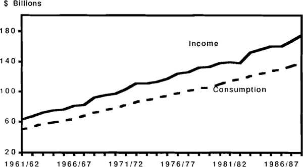
The importance of consumption smoothing behaviour in Australia is illustrated in Figures 28 and 29, showing the relationship between consumption and income. In general there is a strong tendency for consumption to follow income in the long run but to partially smooth out the effects of short-run income fluctuations. The strongest example of this occurred in the 1982/83 recession, when, as was noted in Section 2.1, the private saving ratio fell to its lowest level in three decades. Consumption levels did dip slightly relative to trend in this period, but the time path of consumption remained considerably smoother than that of income.
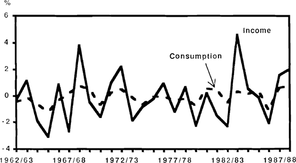
Carroll and Summers (1989) point out that the long-run tendency for income and consumption to grow in parallel is a feature common to a large number of countries. On the face of it, this behaviour is inconsistent with theories that postulate long-run or lifetime consumption smoothing, and the authors argue that the kind of test described above will fail to detect such long-run inconsistencies because they focus exclusively on short-run dynamics. The most obvious way of reconciling aggregate long-run behaviour with the hypothesis of long-run consumption smoothing would be to assert that while individual households smooth their lifetime consumption patterns, the parallel growth of income and consumption is explained by the generational replacement of households with successively higher levels of permanent income. In an attempt to provide evidence on this point, Carroll and Summers cite cross sectional data from the U.S. on consumption and income patterns by age group. The discussion that follows makes use of roughly equivalent data for Australia available from the 1984 Household Expenditure Survey. The data are summarised in Figures 30 to 35.
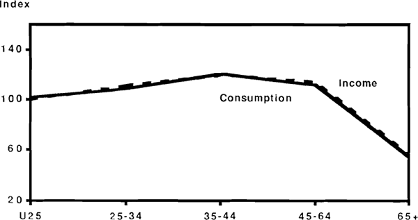
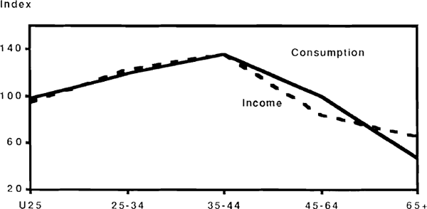
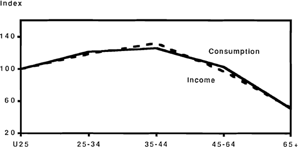
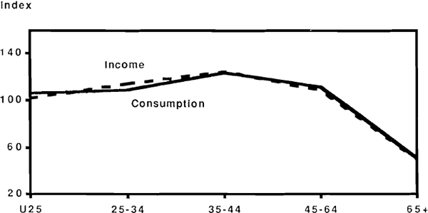
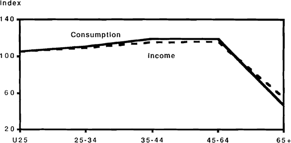
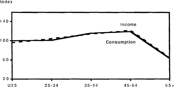
Figure 30 shows the income and consumption levels of households disaggregated by the age of the household head, with income and consumption levels measured as a ratio to the population averages. Thus for example households with head aged 35 to 44 earn 120 per cent of average income, and consume at 121 per cent of the average consumption level. The significant feature of the pattern shown is the close correlation between relative income and relative consumption levels. Households with head under 25 can expect an average growth in relative income of about 20 per cent by the time of reaching the 35 to 44 age group, and yet such households do not appear to dissave in anticipation of that income growth. While this might be explained in terms of inability to borrow against future income, behaviour at the other end of the age range cannot be accounted for in this way. After age 65, both relative income and relative consumption fall by about 50 per cent, with no apparent tendency for this to be smoothed out by saving in the preceding age groups.
The cross-sectional data are thus suggestive of behaviour in which consumption broadly follows the lifetime income pattern. On its own, this fact might conceivably be coincidental: the intertemporally optimal consumption path might happen to coincide closely with the actual time path of income. As evidence against this possibility, Figures 31 to 35 present the same information disaggregated into income quintile groups. Thus Figure 31 shows the incomes earned by the lowest quintile within each age group, expressed as a ratio to the simple average across age groups; if we assume that people remain in the same quintile group for their age-group as they age, then we can interpret the graphs as showing how households income and consumption evolve over time. What these Figures suggest is that differences in the lifetime consumption patterns between groups correspond almost exactly with the associated differences in income patterns. The comparisons are not very exact of course, because households can obviously move between quintile groups during the course of a lifetime. In some cases however, allowing for this possibility exacerbates the inconsistency with lifetime consumption smoothing. For example, a household with head under 25 in the lowest income quintile within that age group, can expect income to grow by 40 per cent, even if it is assured of being in the bottom income quintile of every subsequent age group; the 40 per cent figure is therefore a lower bound on potential income growth, and the suggestion from the data is that this potential income growth is not reflected in current consumption. To take an example at the other extreme, a household in the highest quintile of the 35–44 age group can expect a massive income reduction due not only to the normal life cycle factors, but also to the possibility of moving to a lower quintile when the next age groups are reached. Yet such a household appears on average to consume close to its current income. These features of the data are similar to those reported for the U.S by Carroll and Summers and appear inconsistent with the hypothesis of lifetime consumption smoothing.
To sum up this discussion, the evidence from an examination of consumption smoothing models seems to support two main conclusions. First, there is little or no direct effect of the real interest rate on consumption spending; both income and substitution effects are small or hard to detect. Secondly, consumption smoothing behaviour appears important over relatively short periods (up to two or three years) but probably not over longer periods (decades or lifetimes). Whether this is due to borrowing constraints, short-sightedness, or “rule of thumb” behaviour by consumers cannot be determined from available evidence.[16]
3.2 Saving and Wealth
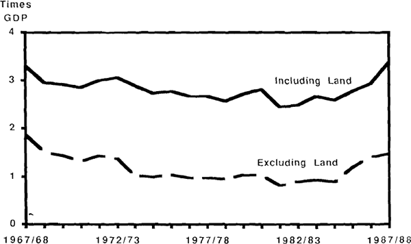
Data on non-human wealth compiled by Horn (1987)[17] and depicted in Figure 36 suggest that the market value of private sector wealth in Australia has risen substantially during the 1980s. From a low of 2.5 times GDP in 1982, the wealth to GDP ratio grew to 3.5 times by 1988. This increase was due almost entirely to valuation effects rather than to accumulation of assets through saving; measured at replacement value, wealth was extremely stable at about three times GDP throughout the decade.
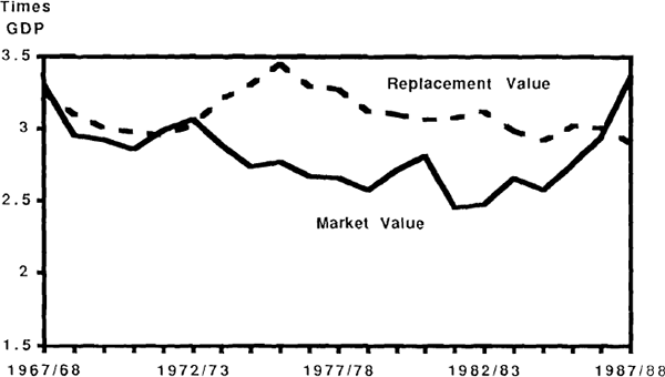
This behaviour of wealth raises a number of interesting questions about how consumers and savers respond to changing wealth levels, and how income and saving should be measured in the presence of large capital gains on the existing stock of assets. Eisner (1988) advocated the inclusion of capital gains in the national accounts as a component of income, which would have the effect of defining saving as the net increment to the market value of wealth. This may be superficially attractive, but there are strong arguments against such an approach. For one thing, capital gains differ from other forms of income because in aggregate (in a closed system) they cannot be realised and converted into consumption. Any attempt to do so would simply drive down the values of the assets concerned. The more fundamental point is that properly speaking, market valuations of wealth represent the discounted value of expected future earnings; changes in the valuation of income-earning assets should therefore be interpreted as revisions to expectations about future incomes, and not as increments to current income itself.[18]
With this interpretation in mind, wealth effects can be logically fitted into the main empirical approaches to the consumption-income relationship which have already been discussed. In the case of Friedman type permanent income models, this involves augmenting the standard distributed lag equation with a wealth term, interpreted as summarising information about future incomes not contained in the lagged income terms. This is essentially the approach taken by Simes and Horn (1986), who used the market value of wealth series referred to above and obtained a wealth coefficient of 1.9 per cent in their consumption equation.
The second empirical framework, based on the intertemporal optimising model, does not require any theoretical modification to allow for wealth effects at all. In principle, both human and non-human wealth are already incorporated in the model through the lifetime budget constraint in the form of expected net income flows; and the testing procedures favoured by proponents of this approach do not require these expected incomes to be measured. Despite this, it can be argued that the rapid growth of market-valued wealth in the 1980s raises an empirical problem for both approaches. On the one hand, the equation estimated by Simes and Horn, using data up to 1986, substantially overpredicts subsequent consumption growth. Alternatively, if one adopts the rational expectations life cycle view, the upward revisions to expected incomes implied by the wealth data should have been matched by a substantial rise in the consumption ratio, which did not in fact occur.
To calculate the increase in consumption predicted by the life cycle theory, one needs to know the proportionate increase which occurred in total wealth (both human and non-human) and hence in permanent income, information which is obviously not known with any degree of accuracy. As a rough guide, if total wealth was valued at 20 times income, then the rise in value of non-human wealth from 1982 to 1988 would have contributed about 5 per cent to the wealth-income ratio which, given a unitary elasticity of consumption, would require a rise of about 5 per cent in the consumption ratio, other things being equal.[19]
Examining a similar puzzle with respect to Japanese behaviour, Hayashi (1989) argued that the problem lay in the definition of wealth; in particular, he showed that land value is not an argument in the solution to the consumer optimising problem.[20] The essence of his argument is that rent on land is both an income and a consumption item, so that an increase in land valuations leaves consumers with just sufficient additional imputed income from land to purchase the same land services as before, at a higher price. In other words, a rise in the real valuation of land represents an income-compensated relative price shift, rather than an increase in real income, and there is no aggregate income effect. Of course, for individual land owners an income effect does exist, but this works by redistributing wealth from renters to owners, rather than creating net wealth in the aggregate.
Hayashi's point seems theoretically sound, and it has considerable practical relevance because land revaluations have made a major contribution to apparent changes in wealth. From Figure 37 it is easy to see that Australia's private sector wealth excluding dwellings has grown much more moderately than the total; land valuation accounted for about half the rise in total wealth which occurred during the 1980s. Hayashi's theory thus makes the relative stability of the consumption ratio in the 1980s much easier to explain.
3.3 Relationship Between Public and Private Saving
Models of consumption smoothing have the property that temporary shocks to disposable income are largely absorbed by changes in saving. One consequence of this property is that exogenous changes to tax rates will tend to affect public and private saving in opposite directions; thus a temporary tax cut reduces government saving, but would be largely saved by the private sector beneficiaries of the cut. As a loose short-run proposition, this would probably have wide acceptance, but proponents of the Ricardian equivalence hypothesis[21] have made the much stronger claim that an exact offset between public and private saving can be expected. The basis of this claim is that government budgets have to be balanced in the long run, so that given spending commitments, governments have discretion to vary only the timing and not the level of taxes collected. This means that tax policies can influence the timing of disposable income receipts but not their discounted present value; hence in a standard life-cycle model they would have no effect on consumption, provided the budget is seen as being balanced within the forecasting and planning horizon of tax-paying consumers.
In reviving this idea Barro (1974) anticipated what he saw as a major theoretical objection, namely that repayment of government debt does not necessarily take place within the lifetime of lenders. Barro offered the counter-argument that taxpayers with operative bequest motives would effectively have infinite planning horizons because they would take account of the expected tax liabilities of their children in determining how much to save for bequests. Not surprisingly this argument has been considered implausible by many economists, and its underlying assumptions have been hotly debated. Bernheim (1989) attacked the idea of making intergenerational transfers central to the model on the ground that it led to absurd conclusions; specifically, one could prove by a seemingly innocuous extension of Barro's assumptions that all government actions are neutral. Other authors have similarly focused on the implausibility of Barro's assumptions about intergenerational transfers, but this issue seems something of a diversion.
The main point is simply to determine whether planning horizons are long enough that individuals would adjust their behaviour to take account of the distant actions of governments. D. Gruen (1988) and Cochrane (1989) both suggested that the information requirements for this to happen are most unlikely to be met by actual consumers; moreover, the efficiency gains to be had from using such information to fine tune the timing of consumption expenditures are probably small. Carmichael (1982) discussed the conditions under which Barro's debt neutrality proposition would hold, and concluded that the extent to which private saving offsets the behaviour of the government could only be determined empirically.
Recent reviews of the empirical literature by Bernheim (1989) and by Leiderman and Blejer (1988) have not uncovered any consensus on the subject. Barro himself does not find this surprising because there is a serious econometric identification problem involved. Both public and private saving tends to move cyclically, rising in booms and falling in recessions, and in order to determine the effect of public sector deficits on private saving, the exogenous component of the public sector position must first be extracted. Due to the difficulty in doing this, Barro (1989, p. 49) prefers to rely on results which “.....exploit situations that look more like natural experiments”. Pursuing this line he cites some evidence from Israel, where large swings in budget deficits have occurred, and a study by Carroll and Summers (1987) on the U.S. and Canadian economies. Both experiences were interpreted as being favourable to the Ricardian equivalence proposition.
Recent experience in Australia also comes close to being a natural experiment lor this purpose, but here the results do not seem favourable. Between 1985/86 and 1988/89, the public sector deficit was reduced by 5 per cent of GDP, and public saving was dramatically increased from 1.1 to 6.6 per cent of GDP. The Ricardian approach would suggest the private sector reduce its saving roughly one for one with the change in public sector saving, but clearly this did not occur; private saving fell only 1.2 percentage points over the period. Further evidence is provided by the longer term evolution of fiscal policy. As was noted in Section 2, private saving ratios were quite stable throughout the 1960s, 1970s and 1980s despite the major swings in public saving after the mid 1970s. Such behaviour suggests very little tendency for private saving to offset changes in the position of the public sector. This has the important policy implication that public saving can be used as an instrument to influence saving at a national level.
One example should be mentioned of a case (similar to examples noted by Kotlikoff (1984)) where something like Ricardian equivalence does seem plausible. The 1987/88 Commonwealth Budget announced a tax measure which imposed a 15 per cent tax on concessional superannuation contributions, with an offsetting reduction in the tax on the accumulated final benefit. This had the effect of raising about $1 billion annually in additional revenue, which would count as an increment to public savings. It can be plausibly argued that fund contributors would not adjust consumption levels to reflect their reduced current after tax incomes, since both their final benefits and current liquidity are unaffected by the change in timing of tax liabilities. Thus private saving would adjust so as to offset exactly the fiscal effect of the current tax increase.
3.4 Demographic Influences
Changes in population growth can be thought to influence saving and investment behaviour in two main ways. First, an increase in population creates a demand for additional capital stock to house and to employ the extra population. Modelling the capital requirements of a growing population, Blanchard (1983) concluded that an increase in population growth will tend to contribute to higher current account deficits because the additional population will generate more investment than saving. Secondly, changes in population growth generally coincide with changes in age composition, and to the extent that saving patterns differ across age groups, this will influence aggregate saving levels.
Details of Australia's population and age structure, including AI3S projections out to the year 2031, are provided in Table 7.[22]
| Age Composition (per cent) |
Growth Rate of Total Population (average to year shown) |
|||
|---|---|---|---|---|
| 0–14 | 15–64 | 65 and Over | % | |
| 1960 | 30.2 | 61.3 | 8.5 | |
| 1965 | 29.5 | 62.0 | 8.4 | 1.6 |
| 1970 | 28.8 | 62.8 | 8.4 | 2.0 |
| 1975 | 27.4 | 63.9 | 8.7 | 1.8 |
| 1980 | 25.3 | 65.1 | 9.6 | 1.2 |
| 1985 | 23.6 | 66.2 | 10.2 | 1.5 |
| 1989 | 22.3 | 66.6 | 11.0 | 1.7 |
| 1996 | 21.5 | 66.7 | 11.9 | 1.5 |
| 2011 | 19.1 | 67.9 | 13.1 | 1.2 |
| 2021 | 18.1 | 65.9 | 16.0 | 1.0 |
| 2031 | 17.6 | 63.6 | 18.9 | 0.8 |
Like a number of other countries, Australia currently has an aging population structure, and this is expected to continue for several decades, primarily as a result of continuation of the low birth rates of the 1970s and 1980s. According to the most conservative ABS projections, the proportion of the population over age 65 will rise from 11 per cent in 1989 to about 19 per cent by the year 2031. At the same time, the young dependency ratio (persons under 15) is expected to fall, as to a lesser extent is the proportion accounted for by the remaining group, the working age population. Under the normal presumption that the over 65 population are heavy dissavers, these projections would imply a declining level of private saving in the out-years of the projection, preceded at some point by a build up in private savings in preparation for that. On the basis of the projections it would seem not unreasonable to expect the savings build up to have begun already, since the working age population ratio is already close to its projected peak. The fact that this has not happened is consistent with the cross sectional data discussed earlier, which indicated very little variation in saving rates across age groups. The implication is that on average, households expect to reduce consumption after retirement rather than to undergo significant dissaving; if such behaviour is maintained, the changing age composition will not have a major impact on aggregate private saving levels.[23]
Arguably one of the major reasons why saving rates vary so little in the years around retirement is to be found in the system of retirement benefit payments. A further discussion of this and related topics will be given in Section 3.5, where it will be argued that the effective tax structure created by these benefits provides a strong incentive for households to match consumption more closely to income than would otherwise be the case. For the moment it is important to note that this effectively shifts a large part of the burden of providing for an aging population from the private to the public sector, although of course policies to encourage private retirement provisions may well prove effective in reversing this. Some idea of the orders of magnitude involved can be gauged by considering the current budgetary cost of pension benefits in relation to the size of the retirement-aged population. Budget estimates for 1989/90 put the cost of age pensions at $8.5 billion, or about 2.5 per cent of GDP. The projected 80 per cent increase in the share of the pension-aged population during the next 40 years could therefore be expected to increase this cost to almost 5 per cent of GDP, assuming the relative value of pensions is maintained. Offsetting this to some extent, there would be some possibility for reduction in the cost of child benefits arising from the trend reduction in the young dependency ratio.
While these changes are not insignificant it is easy to overstate their importance. Compositional changes in the population take place very slowly and their effects may easily be overshadowed by other variables with more immediate impacts. A common finding in overseas studies using simulations of age-specific saving rates[24] is that they have tended to overestimate the effect of demographic changes on aggregate saving when simulated within history. This is not to deny that differences in demographic characteristics may be important in explaining broad differences in saving behaviour between countries. Dean et al. (1989) ranked a cross section of countries by demographic factors thought to influence saving and found that this ranking conformed closely with a ranking of countries by actual saving rates.
A further demographic characteristic which might be thought to have influenced saving behaviour is the tendency for average household sizes to fall, possibly leading to increased expenditure on the housing stock. According to Household Expenditure Survey data, the average number of persons per household fell from 3.1 in 1974/5 to 2.8 in 1984, a fall of 10 per cent. Although perhaps significant for other reasons, the effect on saving through investment in housing seems likely to be quite small: a reasonable upper limit would be to assume this effect has added 10 per cent to dwelling expenditure, which would amount to only about half a per cent of GDP, much smaller than the normal cyclical variation in dwelling investment. Allowance should then be made for two offsetting factors: a likely tendency for smaller households to have smaller incomes and require smaller dwellings; and possible reductions in other consumption expenditures when faced with higher per capita housing costs.
3.5 Effects of the Tax and Benefit System
It was suggested in Section 3.1 that aggregate saving is not very sensitive to changes in interest rates. This might be taken to imply that saving behaviour would be insensitive to tax measures affecting after tax real rates of return, but there are two reasons why such a conclusion does not necessarily follow. First, taxation may have important effects on the allocation of saving without affecting its level; even if there were no substitutability at all between current and future consumption, it is likely there would still be substitution between assets on the basis of differing after-tax rates of return. Secondly, theory suggests that permanent or long-term changes in after tax interest rates have a much larger effect on aggregate saving than do temporary changes.[25] It is the latter which will tend to be picked up (if at all) in evidence from time series data, whereas the relevant features of the tax system are likely to be in place on a much more permanent basis. Effects of taxation on aggregate saving could thus be large but hard to quantify. This Section discusses aspects of the tax and benefit system which might have important effects on the allocation and level of private saving. Other aspects of taxation relevant to investment are discussed in Section 4.2.
In discussing possible distortions in the tax system it is necessary to begin with a view as to what constitutes a neutral system. All taxes are theoretically distortionary (apart from lump sum transfers) and there are two main candidates as benchmarks for neutrality in a weaker sense: a comprehensive income tax, under which real incomes from all assets are taxed at equal rates; and an expenditure tax. In the policy debate there is a certain amount of naive advocacy of the second, on the presumption that it would boost saving by penalising current consumption. This is not strictly correct, since an expenditure tax would be taxing both current and future spending; rather, the effect on saving would operate indirectly by allowing a reduction in marginal tax rates on income from assets. A number of researchers (for example, Summers (1984) and Hall and Rabushka (1985)) have suggested that an expenditure tax would result in higher saving than would be the case under a comprehensive income tax system, but it seems unlikely that a fully expenditure based system with zero income taxes would ever be implemented. For the purposes of this paper it suffices to note that both kinds of tax system require non-discrimination in the taxation of incomes from different assets.
As set out in Table 1, the main vehicles for household saving in Australia are dwellings, nominal interest bearing assets, and superannuation contributions. The tax treatments of returns on these assets vary markedly. Imputed returns on owner-occupied housing, including capital gains, are untaxed. Nominal interest bearing assets on the other hand are extremely heavily taxed in real terms, due to the inclusion of the inflation premium in taxable income; examples with real effective tax rates in excess of 100 per cent are not difficult to construct. (This issue is discussed in more detail by Carmichael at this conference.) The case of superannuation fund earnings is more complex. Prior to changes introduced in the 1983/84 Budget the treatment of superannuation was extremely concessionary; employer contributions were fully deductible, fund earnings were untaxed, and final benefits would be taken as a lump sum taxed at 5 per cent. The 1983 changes raised this tax rate to 30 per cent while maintaining a threshold under which lump sums could be taxed at the more concessional rate of 15 per cent. Changes announced in the 1988 May Statement essentially preserved these features but brought forward the timing of tax payments by introducing a 15 per cent tax on employer contributions and fund earnings, with offsetting reductions to the tax on final benefits.[26] The net effect of these provisions is that saving through superannuation is considerably less favourably treated than before 1983, but is still favourable relative to the alternative of direct holdings of the assets of superannuation funds by households. The concession is higher for higher marginal rate taxpayers.
Looking at the data in Table 1 there can be little doubt that concessional treatment of superannuation earnings has led to a shift in the allocation of savings in that direction. What is more difficult to determine is whether or not this has increased saving in aggregate. The answer to this depends on the extent to which superannuation assets are substitutable for other stores of saving. This question has recently been addressed by Stemp (1988), who cites a number of overseas studies confirming that tax concessions for pension schemes have added to aggregate saving, although by much less than the gross increase in contributions. However, in Australia's case there has been no obvious tendency for private saving to increase over the past decade, despite the fact that life and super contributions increased as a ratio to GDP by over 4 percentage points. This being the case, and taking into account the cost to public revenue of the superannuation tax concessions (recently estimated by Treasury at about $3 billion), it is possible the net effect on national saving may actually have been negative, although of course the counterfactual case is not known.
A possible explanation for the lack of response of aggregate private saving to the increase in superannuation contributions may lie in a consideration of the income distribution of contributors. Based on data from the 1984 Household Expenditure Survey, contributions were provided disproportionately by high income earners, the highest income quintile providing 45 per cent of fund contributions, and the top two quintiles together providing 75 per cent. The significance of this is that high income earners may be less likely than others to be constrained by liquidity, and therefore better able to treat superannuation as a substitute for other assets.[27] On this reasoning the spread of superannuation to lower income earners may well contribute to an increase in aggregate saving in the future. It may be noted in passing that there are no obvious allocational inefficiencies associated with any general tendency for saving through superannuation to increase. As has been noted by EPAC (1988), superannuation funds are an intermediate vehicle for saving flows and should not add to distortions in the final allocation of saving except to the extent that they face different tax incentives to those applying to investors generally. In this respect the case of superannuation differs from that of housing, where favourable tax treatment implies a direct distortion in the final allocation of saving. The incentive to over-invest in housing may however be mitigated by a low elasticity of demand for housing, an issue discussed further by Britten-Jones and McKibbin (1989).
A related, and potentially very important, consideration is the role of publicly funded pension benefits in affecting the incentive to save for retirement. As was noted in Section 3.1, it is a striking feature of the cross sectional data on consumption and incomes by age group that spending in the years around retirement so closely follows the pattern of income. Freebairn, Porter and Walsh (1989), among others, have argued that the incentive to save for retirement in Australia is significantly reduced by the age pension system, citing the high proportion of the pension aged population receiving benefits and the high effective marginal tax rates applying in the range of incomes in which pension benefits are shaded out. A recent statement by the Minister for Social Security (1989) put the number of people receiving age pension benefits at 1.7 million, about 75 per cent of the pension aged population. Further details of the importance of pension benefits in the total incomes of this group are provided in Table 8 below.
| 1 | 2 | 3 | 4 | 5 | Total | |
|---|---|---|---|---|---|---|
| Average Weekly Household Income ($) | 87.92 | 124.62 | 164.72 | 219.97 | 551.72 | 229.48 |
| Proportion of income from government benefits (%) | 95.60 | 82.40 | 87.30 | 62.20 | 14.40 | 47.5 |
| Av. no. of persons per household | 1.004 | 1.33 | 1.84 | 1.99 | 2.43 | 1.72 |
| Proportion of households in group which own house outright (%) | 68.10 | 77.20 | 78.60 | 81.00 | 82.90 | 77.50 |
Source: Household Expenditure Survey, 1984. (ABS 6530.0) |
||||||
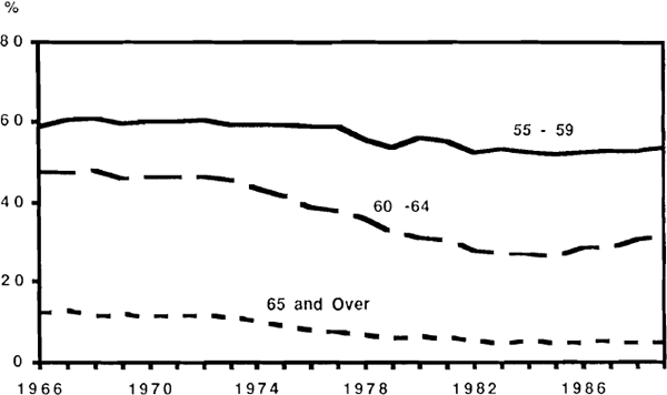
These Figures suggest that a substantial majority (at least 80 per cent) of households have income and spending patterns in the years around retirement which enable them to qualify for benefits, to the extent of forming a majority of their post-retirement income. Stemp (1988) notes the possible adverse consequences of this for labour force participation, particularly when combined with the possibilities for taking concessionally taxed lump sum superannuation benefits as a means of financing earlier retirement. Figure 38 confirms that there has been a dramatic decline in labour force participation for age groups around the retiring age, though this has stabilised and been partially reversed since the mid 1980s. Broadly speaking, the decline in participation by these groups seems to have coincided with a progressive liberalisation of access to age pensions, and increases in their real value.[28]
The question arises as to what is the likely effect of these incentives on aggregate saving levels. A definitive answer obviously cannot be given, but the answer may not be as clearly negative as it would at first seem. Incentives to rely on income-tested government pensions would certainly be expected to reduce saving in the years prior to retirement, but they would also largely eliminate the dissaving phase that would otherwise be expected to follow retirement. The net effect on private saving will be negative only to the extent that average household wealth remaining at end of life is expected to be reduced; and although certain theoretical arguments are available to support such an effect, it hardly seems likely to be large. On the other hand, there is a potentially large effect on government sector balances arising from the provision of pension benefits. Presumably this would have to be offset at some stage (possibly contemporaneously) by taxation, making the pension scheme implicitly self-financing. Such a solution in the longer term would mean higher marginal tax rates, and even if there were no direct effect on aggregate saving rates would probably, as Stemp suggested, have adverse consequences for labour force participation.
Footnotes
Initial wealth is defined as the maximum feasible level of current consumption (achieved by cutting future consumption to zero). Initial wealth will be invariant to the interest rate if there is no non-interest income in the second period. [10]
This point is made by Blanchard and Fischer, 1989. [11]
See for example King (1985). [12]
Deaton (1986) provides a detailed analysis of such issues. [13]
A set of sufficient conditions for this linearisation to be exact is that utility is time additively separable and iso-elastic, and forecast errors are log normally distributed. A derivation of the equation under these conditions is provided by Hansen and Singleton (1983). The equation can also be considered as a linear approximation for a much wider variety of cases. [14]
Estimation of equation (1) for Australia over the period 1968(3) to 1989(4) yielded the result: σ = .05, s.e.(σ) = .08, where σ is the elasticity of substitution. This is similar to the results obtained in overseas studies. [15]
Shefrin and Thaler (1988) propose an interesting “two-self” model in which consumers operate according to various rules of thumb. They argue that such a model can explain many of the empirical anomalies. Other discussions of rule of thumb behaviour are provided by Cochrane (1989) and D. Gruen (1988). [16]
Subsequently updated by Horn to June 1988. [17]
To adopt the latter approach would involve double counting; if expected income in some tuture period was revised upward, the additional income would be counted both in the period when the revision is made, and again when the extra income is earned. [18]
Blanchard (1985) shows that for log utility functions the life cycle model reduces to a simple rule which makes consumption proportionate to wealth. Approximate solutions for the more general case are derived by Campbell and Mankiw (1989). [19]
This argument strictly applies only to land used for housing. [20]
So described because Ricardo (1951) first canvassed the idea, though he did not think it
realistic. Referring to the choice between debt and tax financing of expenditures, he
wrote (p. 186)
“In point of economy, there is no real difference in either of
the modes; [they] are precisely of the same value; but the people who pay the taxes
never so estimate them, and therefore do not manage their private affairs accordingly.
It would be difficult to convince a man........that a perpetual payment of £50 per
annum was equally burdensome with a single tax of £1,000. He would have some vague
notion that the £50 would be paid by posterity, and would not be paid by him; but
if he leaves his fortune to his son, and leaves it charged with this perpetual tax,
where is the difference whether he leaves him £20,000 with the tax, or £19,000
without it? This argument of charging posterity with the interest of our debt, or of
relieving them from a portion of such interest, is often used by otherwise well informed
people, but we confess we see no weight in it.”
[21]
The ABS projections offer several scenarios. The one presented here is the high birth rate, high immigration scenario, which results in the most conservative estimates of population ageing, (source: ABS (1988)) [22]
This conclusion was supported in a recent EPAC paper (1988) which made similar use of the 1984 Household Expenditure Survey information. [23]
Examples include Auerbach and Kotlikoff (1987, 1989), and Wiseman (1989). These and other studies were reviewed by Heller (1989). [24]
Barro (1984) provides an exposition of this result. [25]
Details are obtained from 1983/84 Commonwealth Budget Paper No. 1, and Treasury Economic Statement, May 1988. [26]
King and Dicks-Mireaux (1982) provide empirical support for this proposition. [27]
These changes are reviewed by F. Gruen (1985) who notes that the process of liberalisation began to be reversed after 1978/79 with various steps to tighten eligibility criteria. [28]
