RDP 9103: The Failure of Uncovered Interest Parity: Is it Near-Rationality in the Foreign Exchange Market? Appendix
May 1991
- Download the Paper 251KB
1. Estimation of Ω
The variance-covariance matrix of real relative returns, Ω, is defined as Ω = Et(zt+1−Et(zt+1))
(zt+1−Et(zt+1))′, where  .
To derive
empirical estimates of Ω, we use a sample average of zt for
Et(zt+1). Because US inflation was relatively stable over the sample
period, rather than using actual data, we assume that US inflation is fixed at 0.075% per week
(equivalent to 4% p.a.). Over a week, exchange rate changes – rather than changes in the
US inflation rate – dominate the variance-covariance of relative real returns on a
portfolio of short-term nominal assets. Table 1 displays the empirically estimated
matrix Ω using our 302 weeks of data.[12]
| J | WG | UK | S | A | |
|---|---|---|---|---|---|
| J | .000255 | .000215 | .000180 | .000182 | .000074 |
| WG | .000306 | .000250 | .000248 | .000069 | |
| UK | .000313 | .000203 | .000080 | ||
| S | .000398 | .000042 | |||
| A | .000248 | ||||
2. Alternative examples of near-rationality
In this section of the Appendix, we estimate the cost of two further examples of near-rational behaviour: “covariance blindness”, and small mistakes in the formation of exchange rate expectations.
To estimate the cost of covariance blindness, we assume that our representative investor uses the covariance matrix from Table 1 with all off-diagonal elements of Ω set to zero when choosing shares.
In our final example of near-rational behaviour, the investor makes an unsystematic error when forming exchange rate expectations. Equation (2) is replaced by:
where  are
independent normally distributed errors with zero mean and a standard deviation of 1% p.a.
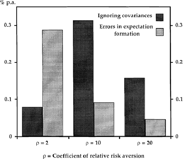
Of course, to estimate the average expected utility derived from these two near-rational strategies, we use the “true” model (which involves using the complete matrix Ω from Table 1 along with equation (2) for exchange rate expectations). Again, the cost associated with a sub-optimal strategy arises from holding inappropriate portfolio shares. Figure 2 shows the costs of these two near-rational strategies.

As in the text, the size of the expected utility costs are small. Assuming ρ = 2, the average cost of ignoring the expected covariance between returns is less than 0.1 %p.a., while the penalty for making errors in the calculation of expected exchange rate changes of around 1%p.a. is about 0.3%p.a. Note, however, that if the expectational errors are substantially larger than l%p.a. on average, the expected utility costs will be correspondingly larger. Taken at face value, survey data on exchange rate expectations (Frankel and Froot (1987)) suggest that expectational biases are often substantially larger than 1%p.a.
Footnote
Prof.W.E.Griffiths pointed out to us that calculating Ω in this manner gives investors the benefit of information they do not yet have. We have established that continually updated estimates of Ω based on available information makes negligible difference to our estimates of the average cost of near-rational strategies. [12]
