RDP 9201: The Impact of Real and Nominal Shocks on Australian Real Exchange Rates 4. Results
January 1992
- Download the Paper 635KB
In order to maximise the available degrees of freedom and to observe short run dynamics monthly data is used. While the preferred measure of the real exchange rate is that using the CPI, Australia does not publish the CPI monthly. Various producer price indices are, however, published on a monthly basis. Below, the producer price index for machinery and equipment is used. Of the available indices this one appears to most closely track the CPI. For the USA and Japan the CPI is used. Unemployment data is seasonally adjusted. All data in this section are taken from the OECD Main Economic Indicators.
There is an active debate over whether or not the exchange rate regime matters for real exchange rate determination. While real exchange rate variability has been greater under the floating regime than under the fixed rate system, one school of thought attributes this to increased volatility in the underlying determinants of real exchange rates.[14] The position taken here is that prices are not instantly adjustable and thus the short-run behaviour of real exchange rates may differ under fixed and flexible exchange rates.
Australia's exchange rate system has undergone considerable change since 1970. At various times the Australian dollar has been fixed in terms of the sterling (prior to December 1971), the US dollar (December 1971 to September 1974) and a trade weighted basket of currencies (September 1974 to November 1976). Between November 1976 and December 1983 the Australian dollar was set on a daily basis in terms of a trade-weighted basket of currencies. Subsequently, the Australian dollar was floated. With an eye to these changes and the desire to maximise the number of available observations January 1977 is chosen as the starting date for the analysis. The sample period runs until July 1990 making a total of 150 useable observations.
For completeness we begin with the results of testing the null hypotheses that each of the series used in this paper have a unit root. Two tests are used: the Phillips-Perron Z(α) (1988) test and the augmented Dickey-Fuller test. The results are reported in Table 2. For both tests a constant is included in the regression. The results are not sensitive to its exclusion or to the inclusion of a time trend. These tests, however, should be interpreted with a deal of caution, as their power depends on the sample length in years. While there are a reasonable number of observations data is only available for eleven years. For a further discussion of these issues see the review in Campbell and Perron (1991).
| VARIABLE | PHILLIPS-PERRON Z(α) | AUGMENTED DICKEY-FULLER | ||||
|---|---|---|---|---|---|---|
| Lags Used in Spectral Density | Number of Lags | |||||
| 6 | 12 | 24 | 3 | 6 | 12 | |
| AUD/USD | 4.52 | 4.81 | 5.00 | 1.70 | 1.49 | 1.65 |
| Δ AUD/USD | 138.4* | 138.5* | 137.1* | 7.68* | 5.23* | 3.57* |
| AUD/YEN | 3.45 | 3.75 | 3.79 | 1.72 | 1.65 | 1.46 |
| Δ AUD/YEN | 162.1* | 178.1* | 179.4* | 5.79* | 3.99* | 3.42* |
| Aust. Unemploy. | 4.65 | 5.86 | 6.19 | 1.99 | 2.29 | 1.58 |
| US Unemploy. | 2.75 | 3.97 | 4.30 | 1.37 | 1.93 | 1.50 |
| Japan Unemploy. | 6.61 | 7.21 | 9.44 | 1.60 | 1.32 | 1.25 |
| Critical Values: | ||||||
| 5% | 13.9 | 2.89 | ||||
| 10% | 11.1 | 2.58 | ||||
|
* indicates that the unit root null is rejected at the 5 per cent level. The entries for the Phillips-Perron test are the Z(α) statistic and for the augmented Dickey-Fuller they are the “t-statistic” for the test that β=0 (see below). The Phillips-Perron test is based on estimating the following equation and testing H0 : α=1: |
||||||
To test H0, the Z(α) statistic is formed as follows:
where is an  estimate of the spectral density at frequency zero of v
and
  . To
estimate the spectral density at frequency zero the Newey-West (1987) estimator is used. Slight
modifications of the test statistic are required when the constant is excluded or a time trend
is added. The augmented Dickey-Fuller test is conducted by estimating the following equation and
then testing H0 : β=O.
The distributions of both the Phillips-Perron and augmented Dickey-Fuller test are given in Fuller (1976) (Tables 8.5.2 and 8.5.1 respectively).
At standard significance levels it is not possible to reject the null hypothesis that the two real exchange rates have unit roots. This tends to support the view that there are shocks to the real exchange rate which have permanent effects. The hypothesis that changes in the real exchange rates have unit roots is overwhelmingly rejected. The assumption that changes in the real exchange rate are stationary thus seems appropriate. These results are not sensitive to the test employed or to the number of lags used. Similar results for a number of currencies are reported in Adler and Lehmann (1983) and Abuaf and Jorion (1990).[15]
The results for the unemployment rates are more problematic. In all three cases it is not possible to reject the null hypothesis that the unemployment rate has a unit root. This is surprising in light of previous work on the stationarity of the unemployment rate. In the seminal study on unit roots, Nelson and Plosser (1982) found that the USA unemployment rate was the only stationary variable of the 14 macro variables examined. Perron (1989), in his recent work, does not even test the unit root hypothesis for unemployment arguing that “there is general agreement that it is stationary”. Campbell and Perron (1991) also argue that the seasonal adjustment procedure often creates a bias toward non-rejection of the unit root hypothesis. The results in the above table, are therefore viewed not as a rejection of the stationarity assumption, but as indicative of a lack of power of the tests using monthly data over the period used in this study. While this interpretation may leave one who is hostile to the stationarity assumption unconvinced, the assumption that shocks which have a permanent effect on the unemployment rate have been unimportant over the sample period examined in this paper, appears reasonable. If the unemployment rate is in fact non-stationary, then the techniques used in this paper are inappropriate as the Wold moving average representation of χ as defined does not exist.
The dynamic responses of the system to the various shocks are examined first followed by an examination of the variance decompositions.
(a) Dynamics
The dynamic responses are broadly consistent with those suggested by the Dornbusch/Mussa model. Real shocks which temporarily reduce domestic unemployment are associated with a permanent real appreciation with the long-run effect being greater than the short-run effect. Nominal shocks which cause a temporary fall in unemployment lead to a temporary real depreciation. There also is evidence of an important international transmission of nominal disturbances in Japan and the United States to Australia. Unfortunately, the bootstrap standard errors are large in a number of cases making strong inferences difficult. Rather than clutter the figures these standard errors are reported in the Appendix for selected lags.
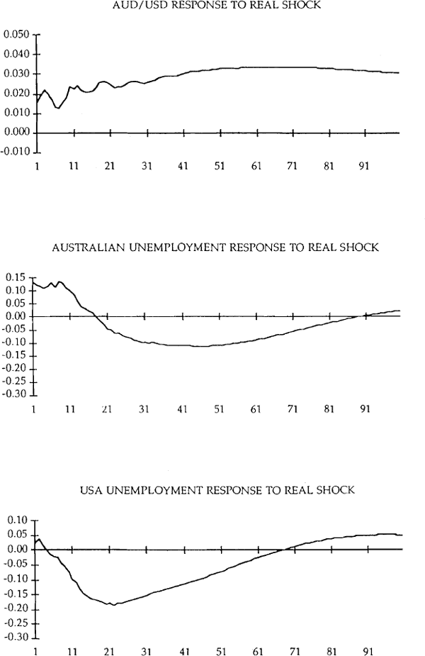
The dynamic responses of the three variables to the real shocks are shown in Figure 1 for the case where the Japan is the foreign country and Figure 2 for the case where the USA is the foreign country. In these and subsequent figures the horizontal axis is time in months.
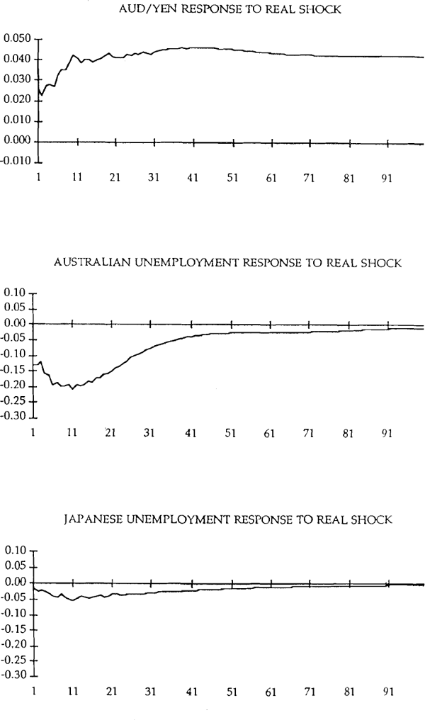
Consider Figure 1 first. As predicted by the Mussa model, the impact effect of a real shock is smaller than the long run equilibrium effect. The impact of the real shock reaches a maximum after some 36 months, although most of the appreciation is completed within 10 months. The final long run effect is approximately 1.6 times the size of the impact effect.
The shock which permanently appreciates the real AUD/YEN rate reduces unemployment in Australia. This is consistent with the impact of productivity shocks in the traded goods sector reducing unemployment temporarily. The maximum employment effect is reached after 6 months. It is sustained around this maximum level for a further 12 months, after which the favourable employment effects of the shock gradually disappear as wages and prices are bid up. After four years the Australian employment response has disappeared. The assumption that there is no long-run employment effect does not appear to be violated.
Japanese unemployment also falls in response to a real exchange rate shock which depreciates the Yen against the Australian dollar. The effect is, however, extremely small.
We now examine the results when the US dollar is the foreign currency. As is the case with the AUD/YEN, the long-run response of the AUD/USD to the real shock is considerably greater than the impact effect. After 48 months the change in the level of the real exchange rate is 1.8 times the initial change. Little additional change takes place after this time.
In contrast to the results for the AUD/YEN rate, Australian unemployment initially increases in response to the real shock which appreciates the AUD/USD real exchange rate. The increase in unemployment is, however, unwound over the next 12–18 months. Unemployment continues to fall out to 36 months after which it gradually returns to its level before the real shock. Two possible explanations for the initial increase in unemployment exist. The first is that at least in the short run there is real wage rigidity in terms of Australia's exports to the USA. There is, however, little evidence that nominal wages increase instantaneously in response to a change in traded goods or export prices. The second explanation is that provided by Blanchard and Quah (1989) who noted a similar response in USA unemployment following a productivity shock which permanently increases output. They argue that nominal rigidities can explain why in response to a productivity shock aggregate demand does not initially increase to match the increase in output needed to maintain output constant. In the medium term real rigidities act to reduce unemployment.
A difficulty with this rationalisation of the results is that when Japan was used as the foreign country we saw a somewhat different response pattern for Australian unemployment. While the declining unemployment after the initial effect is characteristic of both cases the impact effects are different. One would expect that the same factors would be at work in the two cases and thus the responses would be similar.
This lack of similarity in the results for the AUD/USD and AUD/YEN suggests the need to look again at the assumptions underlying the estimation technique. One of the key assumptions is that the disturbances are uncorrelated at all leads and lags. This assumption does not restrict the channels through which the various disturbances effect unemployment and the real exchange rate; however, it is critical that the same underlying data generating process operated through the entire period. Macfarlane and Tease (1989) argue that for some of the floating period the relationship between the exchange rate and interest rates was dominated by a policy reaction function from the exchange rate to interest rates. For example, on occasions when the exchange rate depreciated, the authorities tightened monetary policy. If the deprecation was the result of a real shock in the first place then an induced monetary policy response makes the orthogonality assumption questionable. More importantly Macfarlane and Tease (1989) suggest that the policy reaction function may have changed over time thus altering the data generating process. Given that the exchange rate against the US dollar has typically been the primary focus of attention it seems reasonable to assume that any policy reaction function is heavily weighted towards the US dollar. This clouds the interpretation of the results achieved using the AUD/USD rate and may well be responsible for the different results achieved using the two exchange rates.
In response to the real shock which causes a permanent depreciation of the US dollar against the Australian dollar, United States unemployment falls considerably. The effect reaches a maximum after about 18 months and has all but disappeared after 4 years. Above we have assumed that prices in terms of domestic goods were sticky. If instead wages and prices are sticky in terms of tradeables, a negative productivity shock in the US tradeables goods sector would depreciate the US dollar and would cause unemployment to fall as the wage in terms of non-tradeables falls.
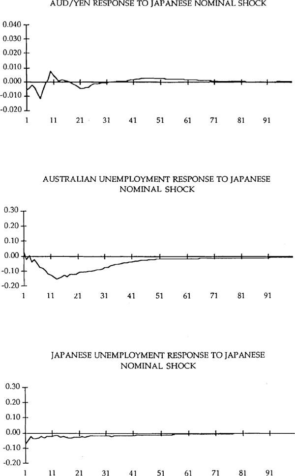
The dynamic responses to the Australian and foreign nominal shocks are shown in Figure 3 for the case in which Japan is the foreign country and Figure 4 for the case in which the USA is the foreign country. First consider Figure 3. The Australian nominal shock has the traditional hump-shaped effect on domestic unemployment. The effect peaks after about 9 months and has vanished after 3 years. These results are similar to those for demand shocks in Blanchard and Quah's decomposition of USA unemployment and output dynamics. As they note, this pattern is consistent with the traditional view of the dynamic effect of aggregate demand on employment in which movements in aggregate demand build up until adjustment in wages leads the economy back to the full employment equilibrium.
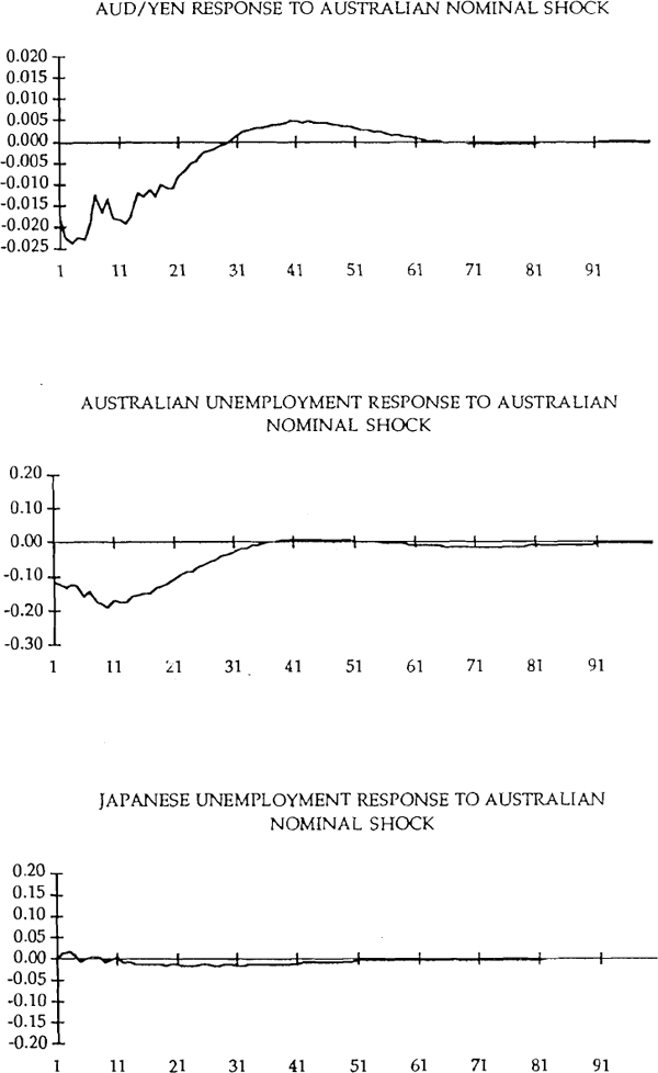
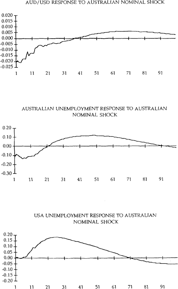
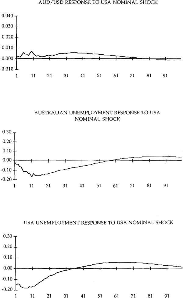
Recall that the Dornbusch/Mussa model predicts that a nominal shock which reduces unemployment causes an immediate real depreciation. This prediction appears to be borne out in the data. The depreciation is gradually worked off over time. After five years the real exchange rate has returned to its initial level, although after 2 years most of the real depreciation has been reversed. There does, however, appear to be some overshooting of the real exchange rate on its way back to its initial level. As expected, Australian nominal shocks have essentially no effect on Japanese unemployment. Of the three shocks, the Japanese nominal shock has the strongest effect on Japanese unemployment. The effect is, however, relatively small. The effect of expansionary Japanese monetary policy on Australian unemployment is also initially very small. It, however, increases over time to reach its maximum effect at the 12 month horizon. Substantially lower unemployment in Australia is sustained for 3 years, suggesting a strong international transmission of Japanese shocks to Australia.
Turning to the AUD/USD rate we see a broadly similar response to the Australian nominal shock that we saw for the AUD/YEN rate. Most of the real depreciation is worked off within two years and there is some suggestion that the real rate overshoots on its way back to its initial level. The favourable employment consequences of the shock last for some 12–18 months after which unemployment appears to be slightly above its equilibrium level for a period of time. The most troubling aspects of the results is the response of US unemployment to the Australian nominal shock. One would expect there to be little, if any, response of US unemployment to this shock. For the first 6 months this is indeed the case, however, the US response gradually increases to be quite sizeable after 2 years. While the effect is larger than expected, an analysis of the variance decompositions for US unemployment shows the Australian nominal shock to account for a relatively small share of the variance.
There again appears to be an important international transmission of shocks with favourable employment consequences in the foreign country to Australia. While the initial effect is small, the impact grows steadily for 12 months and is sustained for a further 12–18 months.
(b) Variance Decompositions
An assessment of the relative importance of the three shocks at various horizons can be gained by examining the proportion of the variance of the forecast error at the relevant horizon which is accounted for by each of the shocks. Define the k month ahead forecast error in the level of the real exchange rate as the difference between the actual value and its forecast from (4), k months earlier. This forecast error has three components: real shocks over the last k periods, Australian nominal shocks over the last k periods and foreign nominal shocks over the last k periods. The variance decompositions for the real exchange rates and the Australian unemployment rates are presented in Tables 3 and 4 respectively. The numbers in parenthesis are standard deviations calculated using the bootstrap technique discussed in Section 3.
| HORIZON (months) |
PERCENTAGE OF VARIANCE DUE TO: | |||||
|---|---|---|---|---|---|---|
| REAL SHOCK | AUSTRALIAN NOMINAL SHOCK | FOREIGN NOMINAL SHOCK | ||||
| Foreign Country | Foreign Country | Foreign Country | ||||
| USA | JAPAN | USA | JAPAN | USA | JAPAN | |
| 1 | 36.6 (22.8) |
64.9 (24.4) |
63.2 (22.5) |
31.6 (27.4) |
0.2 (0.3) |
3.4 (16.4) |
| 2 | 42.4 (27.2) |
56.8 (23.9) |
57.0 (25.6) |
40.4 (26.1) |
0.6 (1.6) |
2.8 (16.3) |
| 3 | 46.4 (28.1) |
57.0 (23.7) |
53.4 (25.8) |
41.2 (25.3) |
0.4 (2.3) |
1.8 (16.4) |
| 6 | 44.6 (27.0) |
59.1 (22.6) |
53.8 (25.6) |
37.2 (21.6) |
1.5 (1.4) |
3.7 (15.7) |
| 12 | 53.8 (17.8) |
73.3 (20.5) |
43.8 (17.4) |
24.5 (16.5) |
2.4 (0.4) |
2.2 (17.1) |
| 24 | 72.0 (9.0) |
84.1 (17.6) |
26.2 (9.0) |
14.7 (10.7) |
1.9 (0.2) |
1.2 (14.5) |
| 60 | 89.0 (2.2) |
94.0 (11.8) |
8.9 (1.8) |
5.5 (5.1) |
2.0 (0.4) |
0.5 (8.8) |
| 150 | 95.0 (1.6) |
97.5 (5.6) |
4.2 (1.2) |
2.3 (2.1) |
0.8 (0.4) |
0.2 (4.3) |
| HORIZON (months) |
PERCENTAGE OF VARIANCE DUE TO: | |||||
|---|---|---|---|---|---|---|
| REAL SHOCK | AUSTRALIAN NOMINAL SHOCK | FOREIGN NOMINAL SHOCK | ||||
| Foreign Country | Foreign Country | Foreign Country | ||||
| USA | JAPAN | USA | JAPAN | USA | JAPAN | |
| 1 | 55.5 (38.3) |
53.2 (25.5) |
44.1 (27.7) |
43.8 (27.4) |
0.4 (4.5) |
3.0 (11.8) |
| 2 | 58.2 (34.8) |
53.0 (24.4) |
38.8 (25.8) |
44.7 (26.0) |
2.9 (4.7) |
2.2 (10.9) |
| 3 | 57.9 (31.3) |
50.5 (23.9) |
38.2 (22.5) |
48.1 (25.0) |
3.9 (1.2) |
1.5 (10.6) |
| 6 | 46.4 (25.2) |
55.7 (24.3) |
40.1 (20.8) |
42.0 (23.7) |
13.5 (1.2) |
2.3 (12.0) |
| 12 | 35.8 (28.6) |
50.7 (24.0) |
34.4 (13.1) |
38.9 (21.2) |
27.8 (0.7) |
10.3 (14.6) |
| 24 | 24.5 (17.7) |
48.3 (24.4) |
25.5 (7.6) |
33.8 (19.6) |
50.0 (5.0) |
17.9 (17.1) |
| 60 | 33.9 (23.4) |
48.3 (23.9) |
34.7 (12.8) |
30.5 (18.9) |
31.3 (3.2) |
21.2 (17.0) |
| 150 | 34.0 (22.8) |
48.4 (23.9) |
37.2 (11.9) |
30.3 (18.9) |
28.9 (3.6) |
21.3 (17.1) |
We first examine the variance decompositions for the real exchange rates. Recall that by construction the percentage share of the variance accounted for by the real shock must go to 100 per cent as the forecast horizon goes to infinity. However, at short horizons, the importance of the real shock is allowed to, and in fact does, differ across the two currencies. For the AUD/YEN rate, 65 per cent of the variance at the one month horizon is accounted for by the real shock. This compares with a figure of 37 per cent for the US dollar. The foreign shock accounts for a very small share of the variance for both currencies. This leaves the Australian nominal shock to account for much more of the short-run variance of the AUD/USD rate than it does for the variance of the AUD/YEN rate. While nominal shocks play a smaller role in explaining the variance as the forecast horizon increases, they maintain an important role out to at least 2 years. At the 12 month horizon the share of the forecast error variance of the AUD/Australian nominal shock is still 44 per cent. At the two year horizon this share has fallen to 26 per cent. After five years it accounts for less than 10 per cent. At all horizons the nominal shock is less important in understanding dynamics of the AUD/YEN rate than it is for the AUD/USD rate. Unlike the decompositions for the real exchange rates, the estimation technique does not impose any restrictions on the variance decompositions for the unemployment rate. In both the cases when the USA and Japan are taken as the foreign country, the Australian nominal shocks accounts for just over 40 per cent of the variance at the one month horizon. At this short horizon, real shocks account for a slightly higher share of the variance (56 per cent in the case of the USA and 53 per cent in the Japanese case). The foreign nominal shock has relatively little role at the shortest horizons. Its importance, however, increases with the passage of time, reflecting the lag in the international transmission of the disturbance. After 2 years the United States nominal shock accounts for 50 per cent of the variance of the forecast error of the Australian unemployment rate. The comparable figure when Japan is taken as the foreign country is 18 per cent.
Footnotes
Mussa (1986) provides a detailed review of the evidence concerning nominal exchange rate neutrality. He notes that while there are many theoretical models which embody the neutrality hypothesis there is little convincing empirical evidence to support it. [14]
Abuaf and Jorion (1990), however, argue that using a multivariate approach results in considerably weaker support for the unit root hypothesis. Tests for a unit root in nominal exchange rates almost universally fail to reject the unit root null. For tests using daily data see Baille and Bollerslev (1989) and for tests using weekly data see Corbae and Ouliaris (1986) and Meese and Singleton (1982). [15]


