RDP 9207: Indicators of Inflationary Pressure 3. The Data and their Time Series Properties
July 1992
- Download the Paper 403KB
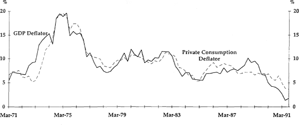
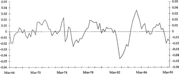
We use two measures of inflation in our analysis. These are the quarterly percentage changes in the implicit price deflators of Gross Domestic Product, which we denote as Δpq; and of private consumption, which we denote as Δpc. These are plotted in Figure 3.[7]
We conduct Phillips-Perron (1988) unit root tests, with four autoregressive lags, to determine the time series properties of our data. Our sample estimation period begins in 1966(2) and ends in 1990(2). Table 1 presents the results of these tests for unit roots in the variables, which, except for the unemployment rate and the rate of capacity utilisation, are expressed in natural logarithms. The evidence from these tests suggest that all variables contain a unit root (i.e. are integrated of order one), except capacity utilisation (cap), which is stationary.[8]
| Variable |  |
Zt |
|---|---|---|
| GDP Deflator (pq) | 1.001 | 0.021 |
| consumption deflator (pc) | 1.002 | 0.282 |
| Gross Domestic Product (q) | 0.990 | −2.372 |
| currency (cr) | 0.998 | −0.947 |
| velocity of currency (v) | 0.884 | −1.909 |
| unemployment rate (u) | 0.983 | −1.431 |
| capacity utilisation (cap) | 0.896 | −3.149 |
|
Critical Values: |
||
Each of the I(1) variables is expressed in stationary form in the regressions which follow. For the price deflators and currency, this is achieved by first-differencing. Given the non-stationarity of q, v, and u it is not possible to estimate q*, v*, and u* using simple trends. Instead, we use the Hodrick-Prescott filter (Prescott, 1986) to construct these variables. This filter decomposes a series into permanent and transitory components. It does so by selecting a trend path τt (permanent component) which minimises the sum of squared deviations from a series yt subject to the constraint that the sum of squared second differences be sufficiently small i.e.
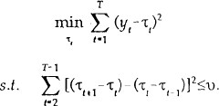
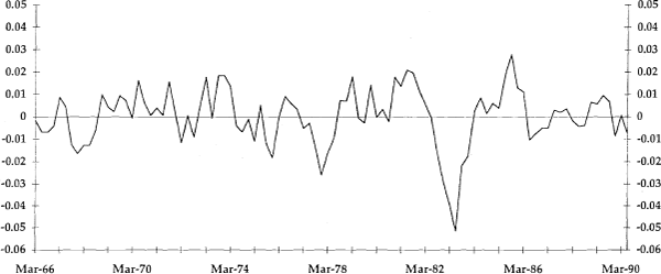
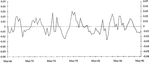
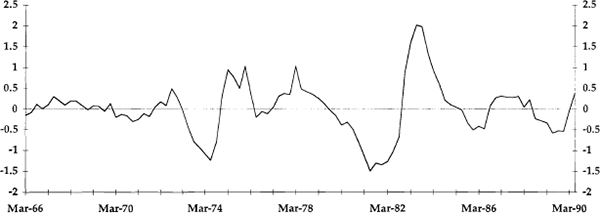
where υ is a constant that determines the smoothness of the trend path. The transitory components are the deviations from the trend, yt − τt. These are plotted in Figures 4 to 7 as the q, v, p and u gaps, respectively. All of these variables have a mean value of zero, by construction.
Footnotes
Δpc cannot be used when evaluating the P* model, since this model is based on the definition of velocity as nominal GDP per unit of money. However, we can use the output gap model (a special case of P*) to forecast Δpc. [7]
We also tested the hypothesis that each variable contains two unit roots i.e. that there is a unit root in the first differences. This hypothesis was decisively rejected on every occasion. [8]