RDP 9207: Indicators of Inflationary Pressure 2. Indicative Models of Inflation

Our base model is an autoregressive representation in which inflation depends solely on past inflation:

where p is the log of the price level, Δp is the rate of inflation, and ε_t is an independent and identically distributed error.

This is the model against which models containing various indicator variables can be compared. These are described in turn:

(a) P^*

P^* is defined as the price level consistent with the current money stock and equilibrium in the economy's goods and financial markets. A value of P^* in excess of the price level P indicates that the price level will increase as the economy moves toward equilibrium.

The concept of P^* can be made operational in the following way. Consider first the identity which defines the velocity of money:

where V is velocity, P is the price level, M is the money supply and Q is real output.

Denoting capacity output as Q^* and trend velocity as V^*, P^* can then be defined:

From (2) and (3), the price gap is defined as the sum of the velocity gap and the output gap, with logarithms of variables in lower case notation:

The inflation rate between periods t and t−1 is assumed to be a linear function of the price gap existing in t−1, plus a distributed lag of past inflation rates:

Alternatively, we can specify the inflation process as

where the price level gap has been partitioned into a velocity gap and output gap.

The P^* model can be interpreted as a generalisation of both Keynesian and monetarist theories of inflation. Inflation in most Keynesian models is determined by past inflation, due to inertia, and the output gap, due to price stickiness (Gordon 1990). In monetarist models, an increase in the money supply temporarily depresses velocity below its trend. This leads to an increase in spending, in turn leading to higher prices until velocity has reached its trend and equilibrium is restored (Hallman et al. 1991). The model given by equation (6) can thus be restricted to three more specialised models. These are the price gap model (α₁=α₂), a Keynesian model (α₁=0), and a monetarist model (α₂=0).

One practical problem in the estimation of the P^* model is that since trend output, q^*, and trend velocity, v^*, are not observed, estimates of these variables need to be constructed. Another issue is the choice of monetary aggregate which is posited to anchor the price level. In the literature, this choice has turned on which aggregate has had the most stable velocity. Hallman et al 1991, in their study using data from United States, choose M2 because, at least since 1955, its velocity has been (more or less) stable, with no trend. However, while this condition is sufficient for the choice of monetary aggregate, it is not necessary. Velocity can have a trend (either deterministic or stochastic) and yet P^* can still be useful as indicator model, provided that the process generating the trend is stable.

Finding a monetary aggregate with this property is no easy task using Australian data because both financial liberalisation and changes in transactions technology have substantially altered the velocity of most of the monetary aggregates in recent years. Moreover, in some cases, this has been not just a once-and-for-all effect, as continuing product innovation is likely to see ongoing switches in demand between various types of assets, distorting the growth rates of particular types of money. Very narrow definitions of money have, however, probably been least affected by these changes.^[1] Accordingly, we focus on currency, defined as the value of notes and coins held by the non-bank public.

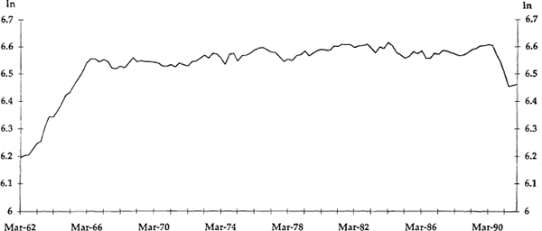
Figure 1 plots the quarterly velocity of currency over the period 1962(1) through 1991(4). Evidently, structural breaks to velocity occurred in the second quarter of 1966 and the third quarter of 1990. Velocity rose substantially until early 1966, and then increased slowly until the second quarter of 1990. This was followed by a sharp fall in the velocity of currency which abated only in the December quarter of 1991.^[2]

What is not clear from Figure 1 is whether velocity followed a deterministic or stochastic trend (contained a unit root) during the period in which it was stable. Clearly, this issue needs to be resolved before we can estimate v^*. If v was trend stationary, v^* can be simply estimated as a (possibly non-linear) time trend. If v^* contained a stochastic trend, it must be calculated in some other way. The same considerations apply to the calculation of q^*.

(b) Other Variables

We also test the usefulness of a number of other variables as indicators of inflationary pressure by estimating an equation of the form

where x is the indicator variable.^[3] These variables are^[4]:

(i) Cyclical Unemployment

The output gap model can equivalently be represented as x = u-u^* where u is the rate of unemployment, u^* is the non-accelerating inflation rate of unemployment (NAIRU), and so u-u^* is the rate of cyclical unemployment. Thus if unemployment exceeds the NAIRU, due to say, a tightening of monetary policy, the rate of inflation is expected to decline.^[5] Empirical implementation of this model requires estimates of u^*, since only u is observed in the data.

(ii) Capacity Utilisation

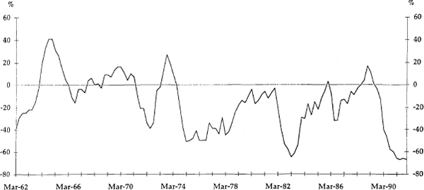
Similar in spirit to the output gap model is a model in which the rate of capacity utilisation is an indicator of inflationary pressure. To measure capacity utilisation we use data from a survey conducted by the Confederation of Australian Industry and Westpac in which manufacturers are asked whether they are working below, at or above normal capacity. The percentage difference between those who say they are working above and below normal capacity is our measure of capacity utilisation. Capacity utilisation is plotted in Figure 2.

(iii) Currency

While the level of currency anchors the price level in the P^* model, its rate of growth can also serve as an indicator of inflation. This is not necessarily because changes in the growth rate of currency cause changes in the inflation rate; however, they might be indicative of such changes. This is so because currency in Australia (and every other developed country) is supplied on demand. An exogenous inflationary shock will to lead to an increase in nominal expenditure; the consequent increase in the demand for currency might then be an indication of nascent inflation.

Another potential leading indicator of inflation that has received increasing attention recently is commodity price inflation (Boughton and Branson 1988, Boughton, Branson and Mutardy 1989, Flood 1989 and Rasche, 1991). Because commodities are traded in competitive markets, unencumbered by long-term contracts, commodity prices are thought to react quickly to fundamental developments, and so commodity price inflation might be a good indicator of embryonic inflationary pressure more generally. However, since commodity prices are set in world markets, and so are unaffected by fundamental inflationary impulses in Australia, commodity price inflation is not likely to be a useful direct indicator of Australian inflation.^[6]

Footnotes

Broad measures of money have been less affected by these change than intermediate measures, such as M3. However, our attempts to use broad money as an indicator of inflation were unsuccessful. [1]

An article in the Reserve Bank of Australia Bulletin, “Recent Trends in Money and Credit” December 1991 suggests some reasons for this decline in velocity. These include new cash transactions reporting requirements and new arrangements for taxing interest, both of which have probably led to an increase in the demand for currency. [2]

We could, of course, specify more than one lag of x in equation 7. However, in empirical implementation, we found that, for every variable, only one lag was significant. [3]

Of course, there are many possible indicators that we do not consider. Blundell-Wignall, Lowe and Tarditi (1992) examine various indicators and their implications for the conduct of monetary policy. [4]

If there is hysteresis in unemployment, the rate of inflation could increase when unemployment is falling, even if it is above the NAIRU. However, we found no evidence of such an effect. [5]

This proved to be the case empirically. In regressions of Australian inflation against various lags of commodity price inflation (not reported), we could never reject the hypothesis that coefficients on the latter were equal to zero. [6]