RDP 9702: The Implementation of Monetary Policy in Australia 2. The Lags of Monetary Policy
April 1997
- Download the Paper 247KB
2.1 The Sources of Monetary Policy Lags
There are six main channels through which changes in interest rates affect economic activity: intertemporal substitution (since interest rates represent the price of expenditure in the present relative to the future), the effect of induced changes in the exchange rate on the tradeable sector, interest rate effects on other asset prices, cash-flow effects on liquidity constrained borrowers, credit supply effects, and the direct effect of changes in monetary policy on expectations of growth (Grenville 1996). Each of these channels – and the interaction between them – makes a contribution to the lags of monetary policy.
To begin at the beginning, however, the first source of monetary policy lags is the delay in pass-through of changes in the overnight cash rate to other interest rates. While the response of short-term money market interest rates is rapid and complete, pass-through to other interest rates such as the deposit and lending rates of financial intermediaries appears to be slower (Lowe 1995). Since intermediaries' interest rates are important determinants of cash-flow, asset prices, and the incentive to postpone expenditure, slow pass-through contributes to the transmission lag from the real cash rate to activity.
Beyond pass-through, an important source of lags arises from the gradual response of investment – both business investment and consumer investment in durables and dwellings – to changes in monetary policy. Adjustment costs associated with changing the level of the relevant capital stock are partly responsible. However, changes in interest rates also affect the incentive to postpone investment when returns are uncertain. The largely irreversible nature of many investments means that there is an option value to waiting to invest in a world of uncertainty (Dixit and Pindyck 1994). When a firm or individual makes an irreversible investment, this option is exercised, eliminating the possibility of waiting for the arrival of new information that might have affected the timing or the desirability of the investment. A change in interest rates affects this option value, and will therefore affect the timing of the investment.
Empirical estimates for the US suggest quite long lags in the adjustment of investment to shocks. For example, Jorgenson and Stephenson (1967) report a mean lag of seven quarters between changes in the rental price of capital and investment in US manufacturing, while Shapiro (1986) estimates that, in response to a shock to the required rate of return on capital, more than half the adjustment in the manufacturing capital stock occurs in the first year, but it takes over four years to be complete.
Turning to asset markets, economic theory would lead one to expect the full implications of a change in monetary policy to be incorporated into asset prices as soon as the change became apparent. In the important case of the exchange rate, however, this does not appear to occur. Thus, for example, Eichenbaum and Evans (1995) find, for the US, that contractionary monetary policy leads to a prolonged gradual appreciation of the domestic currency with the maximal appreciation occurring after two to three-and-a-half years. As a consequence, the exchange rate effects on the tradeable sector of the economy are also gradual and prolonged.
Finally, developments in one sector of the economy are gradually transmitted to other parts of the economy as agents who were initially unaffected by the monetary policy change respond to the altered behaviour of their suppliers and customers. These transmission channels to the wider economy also contribute to the aggregate lags of monetary policy.
2.2 Single Equation Models
Turning to empirical analysis, we begin with single equation models for Australian output. We use a general-to-specific modelling strategy in which insignificant lags of the variables are sequentially eliminated, leading eventually to parsimonious specifications. The models are variants of an earlier model estimated by Gruen and Shuetrim (1994).
We present two models which differ only in their treatment of inflationary expectations. After eliminating insignificant lags, both models take the form,

where Δyt is quarterly growth of Australian non-farm output, rt is the short-term real interest rate, Δft is growth of Australian farm output, yt−1 and wt−1 are the lagged log levels of Australian non-farm output and US output, and εt is a mean-zero error term. Summary results for the two models, estimated by ordinary least squares, are shown in Table 1.[1]
| Variables |
Underlying CPI Model(b) |
Headline CPI Model(b) |
|---|---|---|
| Constant | 24.64** (2.82) |
23.46** (2.64) |
| Real cash rate(c) | −0.035 {0.00} |
−0.036 {0.00} |
| Farm output % change (lag 2) | 0.020* (2.39) |
0.020* (2.26) |
| (lag 4) | −0.020* (−2.23) |
−0.020* (−2.04) |
| Lagged Australian GDP log level | −0.31** (−5.78) |
−0.34** (−5.96) |
| Lagged US GDP log level | 0.38** (6.02) |
0.42** (6.21) |
| US GDP % change(c) | 0.047 {0.00} |
0.061 {0.00} |
| R2 | 0.68 | 0.68 |
| Adjusted R2 | 0.60 | 0.59 |
| Standard error of residuals | 0.56 | 0.56 |
| F-test for joint significance of Australian and US GDP levels | 20.0 {0.00} |
21.3 {0.00} |
| LM test for autocorrelation of residuals: | ||
| First order | 1.49 {0.22} |
0.083 {0.77} |
| First fourth order | 6.58 {0.16} |
4.99 {0.29} |
| Breusch-Pagan test for heteroscedasticity | 20.27 {0.09} |
16.83 {0.21} |
| Notes: (a) The models are estimated by ordinary least squares using quarterly
data over the period 1980:Q3 to 1996:Q1. Numbers in parentheses () are
t-statistics. Numbers in braces {} are p-values. Individual coefficients
marked with *(**) are significantly different from zero at the 5%(1%) level.
All variables in log levels and their differences are multiplied by 100
(so growth rates are in percentages). (b) To derive the real interest rate, inflation expectations are based on the underlying CPI or on the headline CPI. (c) The mean coefficient is reported for the real cash rate and US GDP % change to summarise the coefficients on these variables. The p-values are derived from F-tests of the joint significance of the lags. |
||

The first two sets of independent variables model the influence of domestic variables on output. To control for domestic monetary policy, we use current and lagged values of the short-term real interest rate. With our focus on the length of the lags of monetary policy, we want to allow considerable flexibility in the estimated pattern of influence of monetary policy on output. We therefore use lags 0 to 6 of the short-term real interest rate, rather than eliminating all insignificant lags as we do for other variables.
We assume inflationary expectations are backward-looking. For the underlying CPI model, we use the overnight cash rate set by the Reserve Bank minus underlying consumer price inflation over the past year to measure the short-term real interest rate, while for the headline CPI model, we subtract headline consumer price inflation over the past year.[2] For both models, the coefficients on individual lags of the real interest rate are estimated imprecisely, but the mean of the real interest rate coefficients is negative, as expected, and highly significant (Table 1).[3]
The second set of domestic variables controls for the influence of farm output on the rest of the Australian domestic economy. Although the farm sector accounts for only about 4 per cent of the Australian economy, widespread droughts, and the subsequent breaking of those droughts, lead to large changes in farm output which have multiplier effects on the wider economy.
The rest of the independent variables in the equation control for both the short-run and longer-run effects of US output growth on Australian output. Including lagged log levels in the regression allows for a possible long-run (cointegrating) relationship between the log levels of Australian and US output, with the results providing strong evidence of the existence of this relationship.[4]
The importance of US output for the Australian business cycle, recently highlighted by McTaggart and Hall (1993), appears to arise for several reasons. In the shorter run, links between financial markets (Gruen and Shuetrim 1994; de Roos and Russell 1996; and Kortian and O'Regan 1996), effects on Australian business confidence (Debelle and Preston 1995) and a disproportionately large response of Australian exports to the US business cycle (de Roos and Russell 1996) all play a role. In the longer run, technology transfer from the US seems to be important (de Brouwer and Romalis 1996).
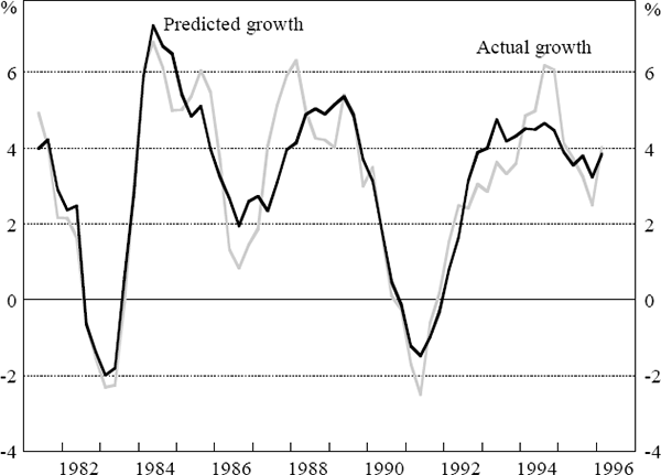
Both model regressions have appealing statistical properties, with no evidence of first-order or first to fourth-order serial correlation and no strong signs of heteroscedasticity. Despite their simplicity, the equations explain a substantial part of the variation in Australian quarterly non-farm GDP growth, with adjusted R2s of 0.60 and 0.59. Both models explain the major features of the Australian business cycle since 1980. Figure 1 shows the results from the underlying CPI model.
2.3 Quantifying the Lags of Monetary Policy
We now return to the lags of monetary policy, and examine the impact on domestic output of a sustained one percentage point rise in the domestic short-term real interest rate. Of course, in conducting this exercise, we should not lose sight of the fact that the domestic real rate is determined in the longer run by the world real rate rather than by domestic monetary policy.[5]
For both models, Figure 2 shows the effect of the rise in the domestic real interest rate on the level of non-farm output, while Figure 3 shows the effect on the year-ended growth of non-farm output. Both figures show point estimates and 90 per cent confidence intervals.[6]
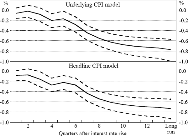
Note: The figure shows point estimates and 90 per cent confidence intervals for the impact on the level of non-farm output of a one percentage point rise in the short-term real interest rate at the beginning of quarter 1.
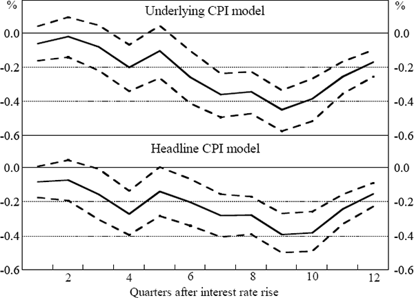
Note: The figure shows point estimates and 90 per cent confidence intervals for the impact on four-quarter-ended growth of non-farm output of a one percentage point rise in the short-term real interest rate at the beginning of quarter 1.
The level of output in either model falls slightly for the first few quarters after a rise in the short-term real interest rate, but the fall is statistically insignificant. Over time, however, the contractionary effect on output gets stronger and becomes increasingly significant. Almost all the effect on the level of output occurs within three years.
It is also clear, however, that the confidence intervals are quite wide. The current real interest rate and its lags are quite strongly correlated, leading to unavoidable problems of multicollinearity in the regressions.[7] As a consequence, it is hard to disentangle the effect on output of the current real interest rate from the delayed effects of the real rate in earlier quarters. In other words, it is hard to estimate accurately the length of the lags of monetary policy.
Another way to highlight this problem is to compare results from the two models on the estimated effect on output growth in the first and second years after a rise in the real interest rate. Assuming inflationary expectations respond to underlying inflation, the fall in output growth is smaller in the first year than in the second (the point estimates are falls in growth of 0.20 per cent and 0.34 per cent), suggesting that the lags in the transmission of monetary policy to output are quite long. Alternatively, assuming inflationary expectations respond to headline inflation, the fall in output growth in the two years is almost the same (the point estimates are 0.26 per cent and 0.28 per cent), suggesting rather shorter lags. The point of this comparison is clear enough: subtle changes in assumptions about inflationary expectations can lead to somewhat different estimated results.
As might be expected, while the point estimates from the two models are different, these differences are not statistically significant. Although the underlying CPI model suggests that the contractionary impact is stronger in the second year, at conventional levels of significance we cannot reject the alternative hypothesis that the impact is in fact stronger in the first year.[8]
An alternative way to summarise the length of the lags of monetary policy is to calculate the average lag length, defined by

where Δmi is the effect on non-farm output growth in quarter i of the one percentage point rise in the real interest rate.[9] Using this formula for the underlying CPI model, the average length of the monetary policy lag is 6.4 quarters; for the headline model, it is a slightly smaller 5.8 quarters. For the reasons explained above, these numbers are again estimated imprecisely, with the 90 per cent confidence interval from 5.1 to 7.7 quarters for the underlying model, and 4.5 to 7.0 quarters for the headline model.
Footnotes
We are faced with the common difficulty in econometrics that we require a timespan long enough to generate meaningful results but not so long that the underlying economic relationships change substantially during the estimation period. With this in mind, we omit the more financially regulated 1970s, and estimate from the financial year 1980/81 to the present, that is, 1980:Q3 to 1996:Q1, giving 63 quarterly observations. For our purposes, the float of the Australian dollar in December 1983 was not an important regime change because, from 1980 to 1983, the exchange rate was adjusted daily via a crawling peg with the US$ and was therefore fairly flexible. For both models, the general specification from which we begin includes contemporaneous and four lags of farm output growth and US GDP growth as well as lags one to four of the dependent variable. A trend term is insignificant when added to either regression. [1]
We also generated estimates of the short-term real interest rate using a survey-based measure of consumers' inflation expectations from the Melbourne Institute survey. The estimation results were qualitatively similar, though the explanatory power of the regression was reduced. Of the two measures of the past inflation used in our estimation, it is unclear which is a better measure of inflationary expectations in the economy. The headline measure is more widely reported but is directly affected by changes in the overnight cash rate (via their effect on variable-rate housing mortgage interest rates); by contrast, the underlying measure, which excludes this direct effect, is a better measure of core consumer price inflation. [2]
As a check of robustness, we also estimated the regression using the yield gap (the cash rate minus the 10-year bond rate) instead of the real cash rate to control for the influence of monetary policy. The results are qualitatively similar, although both the explanatory power of the regression and the significance of this measure of monetary policy are much reduced. [3]
Augmented Dickey-Fuller tests do not reject the hypothesis that the log levels of GDP are stochastically non-stationary I(1) variables (Gruen and Shuetrim 1994). In the regressions in Table 1, the F-statistic for the joint significance of the lagged log levels of Australian and US GDP can be used to test for the existence of a long-run relationship between these variables whether they are I(0) or I(1) variables. It does, however, have a non-standard distribution. For both regressions, we reject the null of no long-run relationship at the 1 per cent level based on critical values tabulated in Pesaran, Shin and Smith (1996). [4]
Since Australia is small in the world capital market, the Australian short-term real interest rate is determined in the long run by the world short-term real interest rate plus or minus a risk premium (assuming no long-run trend in the Australian real exchange rate). Nevertheless, domestic monetary policy determines the Australian short-term real interest rate for long enough to have an important influence on the Australian macroeconomy. [5]
The rise in the real interest rate occurs at the beginning of quarter 1. Therefore, for quarters 1, 2 and 3, the effect on year-ended growth shown in Figure 3 is small partly because the real interest rate has been raised for less than a year. The first year is defined to be from quarter 0 to 4, and the second year from quarter 4 to 8. Since the effect on output of a rise in the real interest rate is a non-linear function of the model parameters, the confidence intervals are estimated using a Monte Carlo procedure described in Appendix A. The point estimates shown in the figures are median outcomes from these simulations, and so they differ very slightly from results derived from the OLS regressions. [6]
For example, the correlation coefficient between the current real interest rate, defined using underlying inflation, and its lags falls from 0.88 for the first lag to 0.74, 0.63, 0.50, 0.34 and 0.22 for the sixth lag. [7]
In about 12 per cent of the Monte Carlo simulations of the underlying CPI model, the contractionary impact on output is stronger in the first year. [8]
To give an example, if the interest rate rise led to an immediate once-off fall in the level of output (and hence a once-off fall in output growth in quarter 1) the average lag length as calculated by Equation (2) would be zero, as required. [9]