RDP 9702: The Implementation of Monetary Policy in Australia 3. Taking Account of the Policy Response
April 1997
- Download the Paper 247KB
3.1 The Problem with Ordinary Least Squares Estimation
Estimating the lags of monetary policy using the approach adopted in the last section has an important drawback. In setting monetary policy, policy-makers do not rely solely on data about the past, but base their decisions also on information about current and expected future developments in inflation and output. From an econometric viewpoint, this renders the real interest rate an endogenous variable, that is likely to be correlated with the current and future residuals in an output equation.
The nature of the problem can be explained using a simple model. Assume that output depends negatively on the real interest rate, while the real interest rate is set on the basis of incoming information about output. In symbols,
where yt is output, rt is the real interest rate, ut and νt are independent error terms and It is information about current output, and is therefore correlated with current output (Et(It ut) = γ). The correlation γ is positive because monetary policy will be tighter when output is expected to be above average.
If the output equation, yt = αrt + ut, is now estimated by ordinary least squares (OLS) the resulting estimate of α is, on average, smaller in magnitude than the true value, α = −1. If the variables ut, νt and It have zero means and unit variances, the ratio Rα of the OLS estimate of α to its true value is Rα = 1−γ/2, which is less than one.[10] Since monetary policy is not set solely on the basis of past information, the strength of its impact on output is underestimated by OLS – at least in this simple framework.
Unfortunately, the problem is more serious than simply underestimating the strength of monetary policy. The ordinary least squares approach also tends to overestimate the length of the lags of monetary policy. To illustrate this point, extend the above model to one in which output depends negatively on both the current and first lag of the real interest rate, while the real interest rate responds to information about output in both the current and next periods. In symbols,
where we have introduced the variable Jt which is information available in period t about output in period t+1, and is therefore correlated with output in period t+1 (Et(Jt ut+1) = δ). Estimating the output equation, yt = αrt + βrt−1 + ut, by OLS leads to estimates of α and β which are, on average, smaller in magnitude than their true values, α = β = −1. If the two errors, ut and νt, and the two information variables, It and Jt, have zero means and unit variances, the ratios Rα and Rβ of the OLS estimates of α and β to their true values are Rα = 1−γ/3 and Rβ = 1−δ/3.[11]
Since information about the current period should be more reliable than information about the future, γ should be greater than δ. Then, while both coefficients are biased towards zero, the bias is likely to be more serious for α, implying that OLS overestimates the length of the lags of monetary policy.
3.2 How Serious is the Bias?
We can extend this analysis to examine the bias in the length of the transmission lags from monetary policy to output estimated in Section 2. To derive empirical estimates of the bias, we need to make assumptions about the correlation between the current real interest rate and the current and future unexplained residuals in the non-farm output equation (Equation (1)).
We assume a correlation coefficient ρk between the current real interest rate, rt, and the unexplained residual in Equation (1) in k-periods time, εt+k, of ρk = γk+1, 0 < γ < 1, k = 0,...,6. This formula embodies the idea used in the simple models above that the correlation is strongest when the output shock and the real interest rate are contemporaneous and falls as the distance in time between the two variables rises. We derive results for values of γ in the range from zero to 0.75.[12]
Assuming a small value for γ implies that the policy-maker raises real interest rates only slightly when information arrives that current growth will be stronger than is implicit in Equation (1), and has virtually no reliable information about future growth other than that predicted by Equation (1). By contrast, assuming γ = 0.75 implies the policy-maker is in possession of good information about both current and future growth shocks, and uses that information to make significant changes to real interest rates.[13]
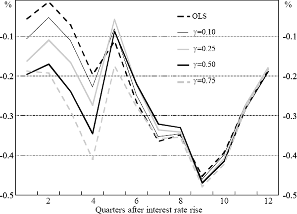
Making these assumptions about the correlations between the real interest rate and growth shocks, we can adjust for the bias in the ordinary least squares estimates generated in Section 2. The details of the calculation are presented in Appendix B, and Figure 4 shows results for the underlying CPI model for four values of γ : 0.1, 0.25, 0.5 and 0.75 (both the size and pattern of the bias are very similar in the two models).

Note: The figure shows, for the underlying CPI model, the estimated impact on four-quarter-ended growth of non-farm output of a one percentage point rise in the short-term real interest rate adjusting for the bias from a correlation coefficient ρk between the current real interest rate and the error in the output equation in k-quarters time of ρk = γk+1, k = 0,…,6, for the values of γ shown.
As for Figure 3, Figure 4 shows the estimated impact on year-ended non-farm output growth of a one per cent sustained rise in the domestic real interest rate. The figure shows point estimates for the OLS regression summarised in Table 1, and for OLS adjusted using the correlations between growth shocks and real interest rates defined above.
The figure displays both of the features revealed by the simple models described earlier. First, OLS underestimates the average strength of the impact of monetary policy on output. And, second, almost all this underestimation occurs for the impact of monetary policy in the first year, implying that OLS overestimates the average length of the lags of monetary policy.
The results in Figure 4 suggest that a moderate amount of correlation between real interest rates and output growth shocks implies that the estimated impact on output growth in the first and second years after a one percentage point rise in the real interest rate is roughly the same, at about one-third of one per cent, falling to about one-sixth of one per cent in the third year. Given the error bands around the original OLS estimates, these numbers are again subject to considerable uncertainty.
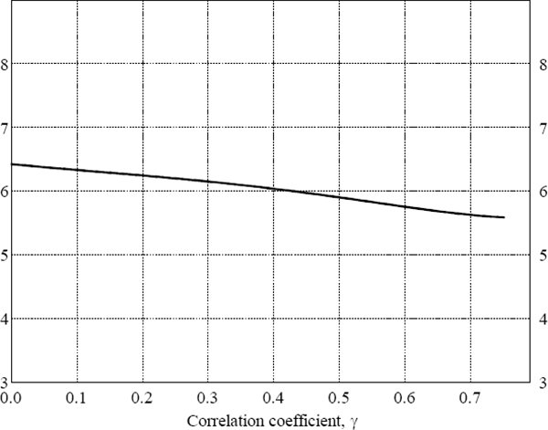
We can also calculate the average monetary policy lag as the parameter γ rises from zero to 0.75. Figure 5 shows the results, which confirm that the average lag length falls with rising correlation between the real interest rate and the unexplained residuals in the output equation. It is of interest to note, however, that the effect is not a very powerful one: plausible values of the correlation coefficient imply only small falls in the estimated average monetary policy lag length.

Note: The figure shows the average lag in monetary policy's effect on output growth for the underlying CPI model, adjusting for the bias from a correlation coefficient ρk between the current real interest rate and the error in the output equation in k-quarters time of ρk = γk+1, k = 0,…,6, for values of γ ranging from zero to 0.75.
3.3 Controlling for the Policy Response using Instrumental Variables
Rather than hypothesising about the correlation between real interest rates and output growth shocks, an alternative approach is to use instrumental variables to control for the forward-looking nature of monetary policy.
Choosing appropriate instruments for the short-term real interest rate is a difficult task, however, made more so by a change in focus of Australian monetary policy in the 1990s with the introduction of a medium-term inflation target. To allow for this change, we assume that there are two monetary policy regimes, old and new, with the real interest rate responding differently in the two regimes.
Rather than conducting an extensive search for instruments, we confine the list to those variables which should have a strong influence on the short-term real interest rate: inflation, π, and the output gap, gap. In the old regime, we also include the current account deficit to GDP ratio, cad, as an instrument because we find that this variable has considerable explanatory power.[14] The variables are lagged to reduce the possibility of correlation between them and the error term in the output equation (1).
For brevity, we again show only the results using underlying inflation (although the results are similar for headline inflation). We use the fitted values from the regression,
to instrument for the contemporaneous real interest rate in the non-farm output equation
(1). The notation implies, for example, that  is the (four-quarter-ended) underlying inflation rate in period t−1
when t is in old regime and 0 when t is in the new regime.
 and
and  are dummy variables for the two regimes and gap is defined as the deviation
of non-farm output from a linear trend. The start of the new regime is the
first quarter of 1990, chosen to maximise the explanatory power of the equation.
The instruments together explain 78 per cent of the variance of the short-term
real interest rate over the estimation period, 1980:Q3 to
1996:Q1.[15]
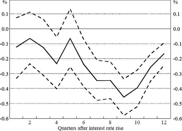
From this instrumental variable (IV) regression, we derive the impact of a sustained one per cent rise in the short-term real interest rate on the year-ended growth of non-farm output. The results are shown in Figure 6. As before, the confidence intervals are estimated using a Monte Carlo procedure described in Appendix A.

Note: The figure shows, for the underlying CPI model, point estimates and 90 per cent confidence intervals for the impact on four-quarter-ended growth of non-farm output of a one percentage point rise in the short-term real interest rate at the beginning of quarter 1.
The results in Figure 6 are not markedly different from the ordinary least squares results using the underlying CPI model in Figure 3. The estimated contractionary impact in the first year is somewhat stronger in the IV regression than in the OLS one, but it is also less precisely estimated. In common with the OLS results, the estimated impact on output growth in the second year is somewhat stronger than in the first year, but the difference is again statistically insignificant.[16]
3.4 Have the Lags of Monetary Policy Changed over Time?
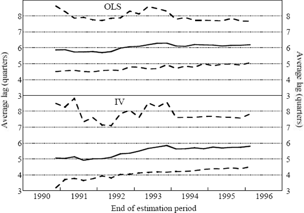
To examine whether the lags of monetary policy have changed over time, we conduct recursive estimation on the underlying CPI model, using both ordinary least squares and instrumental variables regressions. The recursive estimation fixes the starting date at the beginning of the full sample, 1980:Q3, and extends the end of the estimation period from 1990:Q3 to 1996:Q1, one quarter at a time. Figure 7 shows how the average monetary policy lag (defined by Equation (2)) changes as the estimation period is lengthened through the 1990s. As before, both point estimates and 90 per cent confidence intervals are shown.

Note: The figure shows recursive point estimates and 90 per cent confidence intervals for the average lag in monetary policy's effect on output growth for the underlying CPI model, using both OLS and IV estimation techniques.
The results do not suggest any shortening of the lags of monetary policy over the 1990s. As the estimation period is lengthened, the ordinary least squares regressions show a very slight rise in the average monetary policy lag length, while the instrumental variables regressions suggest a somewhat larger rise in the lag length. Needless to say, these results are not statistically significant because the confidence intervals are so wide.
3.5 Comparison with Other Estimates of the Lags of Monetary Policy
Table 2 shows the effect on output growth in the first, second and third years after a rise in the short-term interest rate for a range of models estimated for the Australian and US economies.
| Model | First year | Second year | Third year |
|---|---|---|---|
| Australia | |||
| Current model(b) | −0.35 | −0.33 | −0.18 |
| Murphy(c) | −0.51 | −0.31 | +0.08 |
| TRYM(c) | −0.37 | −0.37 | −0.07 |
| United States(d) | |||
| MPS | −0.20 | −0.70 | −1.10 |
| DRI | −0.47 | −0.53 | −0.13 |
| FAIR | −0.24 | −0.25 | +0.03 |
| FRBSF | −0.55 | −0.19 | +0.04 |
| VAR | −0.64 | −0.26 | +0.08 |
| Notes: (a) For the Australian models, the policy experiment involves raising
the short-term real interest rate, while for the US models, the short-term
nominal rate is raised. Given the sluggish adjustment of inflation, this
difference should not matter much. (b) The results for the current model are those for the underlying CPI model, bias-adjusted assuming γ = 0.5. (c) See Murphy (1995) and The Treasury (Australia) (1996) for a description of the models. Assuming the models are linear for small changes, the results are derived by adding up the impact on output of a series of nominal shocks which together imply a one percentage point rise in the short-term real interest rate for 12 quarters. The results using the TRYM model should in no way be regarded as being Treasury analyses of the effect of a given policy change or as having the sanction of the Treasury, the Treasurer or the Commonwealth Government. (d) The MPS model is maintained by the staff of the Federal Reserve Board, the DRI model is commercially available, the FAIR model is maintained by Ray Fair of Yale University, the FRBSF model is maintained by the Federal Reserve Bank of San Francisco, while the VAR model is a standard vector autoregressive model (see Rudebusch (1995) for further details). |
|||
There is qualitative agreement between the models that output growth falls in both the first and second years after a rise in the short-term interest rate, although there is no such agreement about the third year. Even for the first two years, however, the quantitative estimates differ quite substantially between models.[17] This is simply another manifestation of the technical difficulties associated with estimating the lags of monetary policy.
3.6 Implications for Policy
On the basis of our empirical results, we conclude that output growth falls by about one-third of a per cent in the first and second years after a one percentage point rise in the short-term real interest rate and by about one-sixth of a per cent in the third year, implying that the majority of the effect on growth occurs more than a year after a change in interest rates. These relatively long lags, combined with the problems inherent in forecasting economic growth more than a year into the future, point to the difficulty of trying to use monetary policy to iron-out fluctuations in the business cycle.
Two points are worth making in response to this observation. First, although our discussion has focussed on the response to a once-off permanent interest rate change, monetary-policy-induced changes in the real interest rate are, in fact, temporary. Consider a temporary policy change: a one percentage point rise in the short-term real interest rate that is reversed after a year. The biggest impact of this is in the first year, with output growth falling by about one-third of a per cent. Combining the effect of the interest rate rise and subsequent fall, output growth is then unchanged in the second year, with the policy effect being unwound by one-sixth of a per cent in each of the following two years. The implication is clear enough. The maximal effect on growth of temporary changes in short-term real interest rates is concentrated in the near-term, where useful information is available on expected developments in inflation and output.
Secondly, a key focus of monetary policy is on medium-term price stability. While output is an important leading indicator of inflation, successful pursuit of a medium-term price target does not depend on being able to ‘fine-tune’ the business cycle. Prolonged swings in output can and should be avoided, but the policy lags are long enough, and uncertain enough, that it is futile to try to use monetary policy to fine-tune the business cycle.
Footnotes
The wording in the text is heuristic rather than rigorous. The actual definition
of Rα is Rα = plim / α
where
  is the OLS estimate of α, and plim is the probability limit.
[10]
Again, the wording in the text is heuristic rather than rigorous. See the previous footnote. The bias we refer to in the text is really asymptotic bias. [11]
In general, the correlation between the real interest rate and the unexplained residual depends both on the quality of information available about the unexplained residual and the extent to which policy reacts to that information. The assumption of a falling correlation as the distance in time between the two variables rises could arise either because information is poorer about future residuals, or because policy reacts less to that information. [12]
Assume that the information available to the policy-maker enables him/her to make unbiased forecasts of the current and future shocks to the output equation. Then, for our parameter values, γ = 0.75 means that when the policy-maker has information implying that the level of output will be half a per cent higher than forecast by the equation in each of the next two years, the short-term real interest rate is immediately raised by two-thirds of one per cent. We judge this to be a significant policy reaction. [13]
This does not mean that monetary policy ‘targeted’ the current account, as is sometimes suggested, only that policy responded to changes in demand conditions which were reflected in changes in the current account deficit. [14]
Since policy-makers set the short-term real interest rate partly on the basis of information about current output not available to the econometrician estimating Equation (1), we should expect positive correlation between the errors in Equations (1) and (3). The estimated correlation coefficient between the errors, at 0.08, is positive, but small. [15]
It would be of interest to instrument not only for the contemporaneous real interest rate but also for some of its lags. Unfortunately, however, given the strong correlation between the real interest rate and its lags and the fact that the instruments are not very good, this exercise did not yield any useful information. [16]
In the case of the Murphy model, the stronger contractionary impact in the first year may be partly a consequence of the assumption of uncovered interest parity which implies an initial jump appreciation of the real exchange rate, and therefore a significant contractionary impact on output via its effect on net exports. [17]


