RDP 9802: Systematic Risk Characteristics of Corporate Equity 3. Characterising Systematic Risk

Analysis of the systematic risk associated with equity returns begins by obtaining minimum mean-square estimates of equity betas for each observation, indexed by i for the firm and t for the month. The model is a generalisation of the CAPM type relationship used to discern the systematic risk component in equity returns, β_itr_mt, from the idiosyncratic component, ε_it:

where r_it is the equity return for firm i, r_mt is the value-weighted average return on the NYSE, including all distributions of income such as dividends and bonuses.

How is it possible to estimate the separate equity betas for each observation as is necessary to capture the cross-section and time dimensions of equity betas? The answer is that a substantial structure needs to be placed upon the model defining equity betas. Specifically, the coefficients, γ_it and β_it, are assumed to adjust through time according to the transition equations:

The intercept coefficient, γ_it, is time invariant in the sense that it is not affected by a shock in each period whereas the slope coefficient, β_it, is a random walk process, adjusting by the shock, η_it, in each period. It is assumed that the idiosyncratic shocks to returns are normally distributed with mean zero and variance, . Likewise, the shocks that change the beta coefficient from period to period, η_it, are assumed to be normally distributed with mean zero and variance . Further, Both shocks are assumed to be independently and identically distributed through time and are independent of each other.

From an econometric perspective, Equations (4) and (5) define a state space form that can be estimated using the Kalman filter to extract a sequence of betas for a given vector of hyper-parameters (see Harvey 1989). Equation (4) is the measurement equation and Equation (5) is the transition equation. Constrained maximum likelihood methods are then applied to the log-likelihood function formed from the resulting prediction-error decomposition. The model is an extension of the random walk with noise model in Harvey (1989, p. 37) allowing for an explanatory variable with a time-varying parameter. By imposing this structure on the betas, the problem of estimating betas for every time period is reduced to one of estimating only and . When initialising the Kalman Filter, it is necessary to specify the current ‘state’ of the system. This paper assumes that the initial intercept is zero with a diffuse prior while the beta coefficient is unity with a prior variance of 0.25 which approximately matches the cross-sectional variance of betas around unity observed by Vasicek (1973).

It should be noted that the random walk transition equation for β_it prevents the beta extraction model from imposing any form of mean reverting behaviour. Rather, the equity betas have been estimated under the null hypothesis that betas do not converge. This strengthens the conclusions, drawn in the next section, that betas do exhibit convergence to unity.

A generalisation of the model would allow the intercept to vary over time as well as the equity beta coefficient. This generalisation is rejected by the data which cannot distinguish between shocks to the intercept and the idiosyncratic shocks to returns in the measurement equation, ε_it. Stationary processes for the equity betas were also explored. However, in the majority of cases, the auto-regressive coefficient on the lagged slope coefficient in the state equation approaches unity when maximising the log-likelihood function. While the density of betas appears to be stationary, the samples used for firms are too short and high frequency to capture their mean reversion.

Given estimates of the hyper-parameters and applying the fixed-interval smoother of Jazwinski (1970, pp. 216–217) to condition on the full set of observations, t=1…T, yields estimates of for all observations. The smoothing process is required to ensure that the precision with which betas are estimated is independent of their placement in the time dimension of the sample.

3.1 The Data

The time-varying parameter model described above is estimated for every firm with consecutive data for one year or more. This reduces the number of firms in the sample from 4,343 to 3,992. It also means that inferences from this study are only applicable to firms that survive the first year after their initial public offering (IPO). Using firms with only twelve months of data could give beta estimates that are very imprecise given that 1,004 firms in the sample have between 12 and 60 observations. However, the imprecision in their beta estimates should not lead to evidence of beta convergence. While the imprecision will overstate the mobility of equity betas, it will not bias the results toward beta convergence because of the tight initial prior around unity. The tight prior will tend to force firms with uninformative data to have equity betas that start close to unity and diverge through time.

To implement the beta estimation process, the market return is proxied by the value-weighted average return on the NYSE. In light of Roll's (1977) critique, using the value-weighted average return on the NYSE as a proxy for the market limits the implications of this work for the CAPM. However, this paper does not attempt to advance the literature on CAPM testing. Rather, the estimates of the equity betas are interpreted as measures of covariation between the return on an individual firms' equity and the returns on the equity market. To the extent that these equity betas are related to features of firms, the use of the value-weighted average return on the NYSE does not flaw the analysis.

There are several reasons why using the value-weighted average return on the NYSE is preferable to using more complex measures of market performance. First, managers and investors can easily compare firm performance to that of the value-weighted average return on the NYSE. This makes direct endogenous responses of firms to their equity betas more plausible. More complex characterisations of the market portfolio (e.g. incorporating fixed income assets, real estate and even non-marketable assets) which should be used to test the CAPM, may not be as relevant to the investigation of firm behaviour precisely because they are not easily observed by firms. Alternative covariation benchmarks like that used in Breeden's (1979) consumption CAPM, are also less relevant, despite their sophistication, because of the difficulties in adjusting consumption data to obtain a reasonable measure of consumption flow. A second point in favour of using the value-weighted average return on the NYSE is that Fama and French (1992) report that it yields similar results to using the broader valued weighted equity return on NYSE, AMEX and NASDAQ listed firms.

One way in which this paper differs from the literature testing the CAPM is that betas are constructed using raw, rather than excess, returns. Before presenting these betas, it is worth emphasising how small an effect this has for each firm. Figures 1 and 2 graph the standard errors for the measurement equation and transition equation respectively. They show the estimates computed using raw returns on the horizontal axis against those computed using excess returns on the vertical axis.

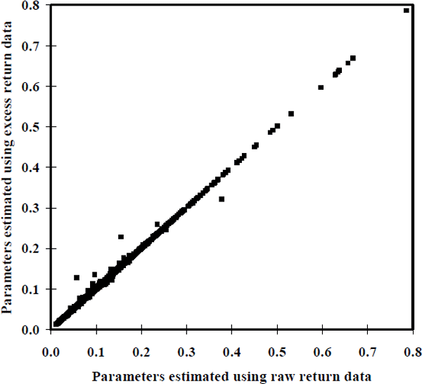
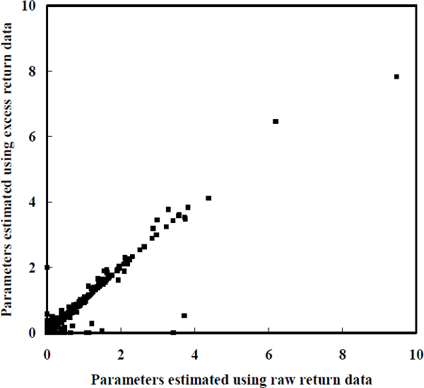
The fact that both of these figures approximately form a 45° line suggests that the choice of using raw or excess returns is not going to influence results significantly. This suggestion was verified by explicitly generating the reported results using excess returns. Raw returns have been made the focus of attention to clarify the interpretation of equity betas as measures of co-movement between firm performance and the performance of the entire equity market. Estimating equity betas using raw returns also de-emphasises any contribution being made to the asset-pricing literature.

3.2 Estimates of the Equity Beta Models

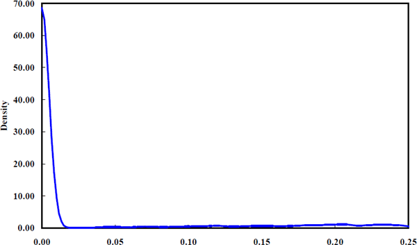
Although reporting the maximum likelihood estimates for each of the firms is uninformative, it is possible to estimate density functions showing how each of the hyper parameters, σ_iε and σ_iη, is distributed across firms. These estimated density functions are shown in Figures 3 to 5. To interpret the density functions, it is important to know how they have been constructed.

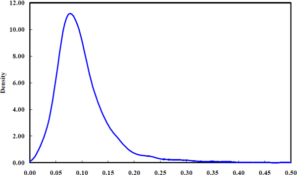
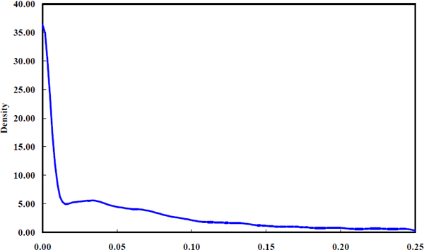
The density functions are estimated by pooling across firms and using non-parametric kernel-density estimation as discussed in Silverman (1986). Intuitively, the density estimate is a smoothed histogram wherein each observation in the histogram is replaced by the kernel function. The kernel function is simply a continuous, differentiable function that integrates to unity. In other words, it is a density function itself. In this paper, the standard normal distribution is used as the kernel function. The individual kernel functions, one for each observation, are integrated to obtain the estimate of the population density from which the sample has been drawn. By replacing each observation with the kernel function, this density estimate is continuous, smooth and it integrates to unity.

Formally the kernel density estimate at x of random variable X is given by:

where, X_i is the ith realisation in the sample, h is the window width, n is the number of observations in the sample and K(·) is the kernel function.

The smoothness of the density estimate depends upon the choice of the smoothing parameter, h, referred to as the window width. This parameter is a scalar value for univariate density estimation. It defines the extent to which the probability mass associated with each observation is smoothed out over the support of the density. The larger the window width the more smoothing occurs in the estimation procedure because each observation is spread over a wider region of the support. In most cases greater smoothing reduces the variance of the density estimate while increasing the bias.

When constructing the density estimates, a subjective approach to window width selection is adopted. The subjective approach is recommended by Silverman (1986) in situations where interest focuses on the shape of the density rather than on applying more formal non-parametric inference techniques. Experimentation suggests that the information content of the univariate density estimates is unaffected over a wide range of window widths.

The estimated density functions in Figures 3 to 5 are suggestive of the range of parameter values obtained across the sample of firms. For example, Figure 3 indicates that for most firms, the standard deviation of idiosyncratic shocks to equity returns is less than 0.15. Likewise, from Figure 4, the shocks to equity betas for most firms have a standard deviation below 0.025. The density functions provide a feel for the location and dispersion of the hyper-parameter estimates. It is clear from Figure 5 that the majority of firms have very low signal-to-noise ratios, σ_iη /σ_iε, implying that betas generally adjust very slowly compared to the overall volatility of equity returns. However, the estimated signal-to-noise density has a substantial upper tail with a few extreme firms having signal-to-noise ratios above one. The hyper parameters in these cases are usually very imprecisely estimated.

3.3 Equity Betas and Other Characteristics of Equity Returns

Additional information about firms' equity returns is provided in the form of densities of equity betas and the standard errors of estimated equity betas. The standard errors of the equity beta estimates are computed directly from the sequence of state variance-covariance matrices obtained for each firm. The data has been arbitrarily broken up into the sub-samples: 1926–50, 1951–75 and 1976–92. A visual comparison of the densities in Figure 6 and in Figure 7 is an informal means of examining the assumption that it is valid to pool observations across the entire time dimension.

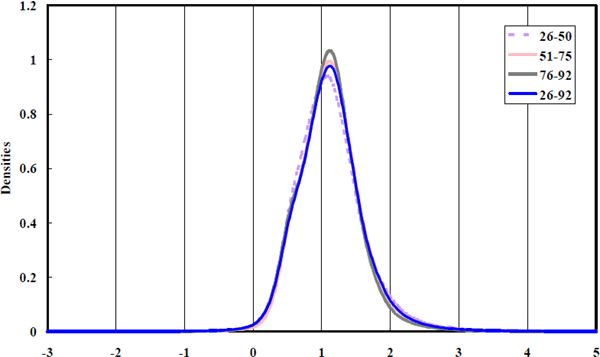
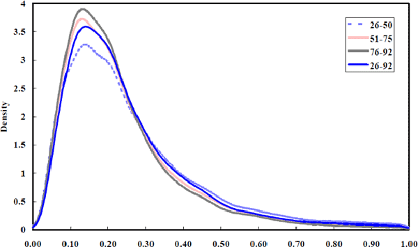
The density functions generated for different time periods are fairly homogenous, confirming the validity of pooling across time. Stability of the densities through time was formally tested using the Kolmogorov (1933) and Smirnov (1939) test for which critical values are tabulated in most textbooks on non-parametric testing methods. These tests contradict the visual message that the densities are similar by powerfully rejecting the null hypothesis that the densities are stable through time even at the one per cent level in a two-sided test. The importance of the rejection of the null hypothesis is difficult to assess because it is driven by the extremely high power afforded by the large dataset. The rejection of the null hypothesis is a common phenomenon with large datasets and is an implication of the fact that null hypotheses are statements of equality that are almost never going to be true.

Figure 6 shows that the vast majority of betas lie between zero and two, though extreme observations are observed on both sides of this range. The concentration of beta estimates around unity is consistent with the statistics on portfolio betas discussed in Fama and French (1992). It is also consistent with the cross-sectional densities described in Vasicek (1973). These consistencies support the validity of the adopted beta estimation methodology.

Figure 7 shows the precision with which betas of individual firms have been estimated. With standard errors averaging 0.25 for the entire sample and having a standard error themselves of 0.13, it is clear that the betas are imprecisely estimated. It should be noted that this lack of precision in individual beta estimates will affect the conclusions to be drawn about beta mobility. This is because, although individual firm's betas may be estimated with substantial error, these measurement errors will be highly correlated through time for given firms. In the extreme case where the measurement error is constant through time, for a given firm, the measurement errors will have no impact on the representations of beta mobility in the next section. As the serial correlation of beta measurement errors declines, the estimated laws of motion for betas will overstate beta mobility. However, it will not lead to an overstatement of the extent to which betas have a tendency to converge to unity given the tight prior around unity imposed on the beta estimation procedure.