RDP 9812: An Optimising Model for Monetary Policy Analysis: Can Habit Formation Help? 6. Accuracy of the Linear Approximation

For computational tractability, all of the computations reported above depend on the linearised approximate consumption function. An important question is how well the linear approximation reflects the underlying nonlinear model from which it is derived.

I present several measures of the approximation's accuracy. First, I solve the nonlinear model (substituting Equation 3 for Equation 6), using the parameters estimated from the linear model, for the standard disinflation simulation of the previous section. As Figure 7 shows, I obtain nearly identical results.^[9]

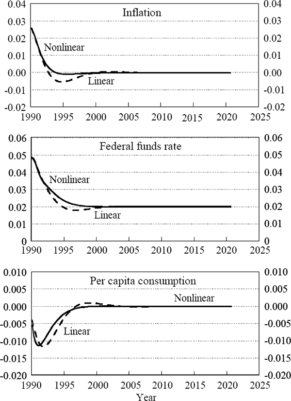
In addition, substituting the linear model's solutions for consumption, income, and real interest rates into the nonlinear first-order conditions, I find that they hold quite well. The maximum absolute error in the nonlinear Euler equations is about 0.01, compared with steady-state marginal utility of about −1. Finally, the estimate of lifetime utility for the disinflation simulation is very similar whether computed using the solution paths from the linear model or from the nonlinear model.

Overall, then, it appears that the linear model provides a very good approximation to the behaviour implied by the nonlinear model.

Footnote

Note that for the nonlinear solution exercises presented here, I use a ‘certainty equivalence’ solution technique that does not compute the stochastic distribution of the endogenous variables via value-function programming. The state dimension of the model would make the computation time for such a method prohibitive. [9]