RDP 2001-09: What do Sentiment Surveys Measure? 3. What Explains Sentiment?
November 2001
- Download the Paper 300KB
It is clear from the previous section that while the existing literature recognises that sentiment may be endogenously determined, it places most emphasis on using sentiment variables to predict or forecast consumption and other activity measures. However we begin our study with a different focus. This section takes up the basic, but fundamental, question of whether sentiment responds consistently to prior economic information. This section also provides the foundation for later investigations of the predictive ability of sentiment indices.
3.1 What is Sentiment?
While the results of sentiment surveys may be well known, their methods of construction are more obscure. This section presents some details on the construction of each index we use. The construction of all the survey indices is similar. Respondents are asked a number of questions about economic conditions, their responses are categorised as: i) up/positive, ii) no change/don't know or iii) down/negative. An index for each question is constructed as the ‘net balance’ where the proportion of negative responses is subtracted from the proportion of positive responses. The overall indices are constructed as an average of the net balance for a number of questions. This method of construction ignores a number of features of the data and there may be alternative methods that would yield more informative indices. For example, abstracting from adding up constraints, the proportion of people holding a ‘no change’ opinion has no effect on the final index yet could, arguably, contain information on people's expectations. We consider the effect of alternative construction methods a little later.
We now turn to the specific measures of confidence we use. To investigate business sentiment, we focus on the ‘Business Confidence’ and ‘Business Conditions’ indicators from the NAB Quarterly Business Survey. The Business Confidence index is a net balance of responses to the question:‘Excluding normal seasonal changes, how do you expect business conditions facing your industry to change in the next three months?’ The Business Conditions index is an unweighted average of three net balance indices expressing respondents' expectations about changes in their firms' trading performance, profitability and number of employees over the past quarter. Neither index is seasonally adjusted as the questions are couched in seasonally adjusted terms. Each series extends from 1989:Q3, when the NAB survey started, to 2001:Q1.
To analyse consumer sentiment, we use the Westpac-Melbourne Institute Index of Consumer Sentiment and the Roy Morgan Consumer Confidence Rating. Until 1990 there was only one such measure, drawn from a single survey conducted jointly by the Melbourne Institute and Roy Morgan. A falling out since then has led to the production of two indices, although the Westpac-Melbourne Institute index receives much broader media attention. Both indices are unweighted simple averages of five component indices, each of which is calculated by adding 100 to a net balance of positive minus negative responses to a specific question. The five questions cover respondents' evaluations of: (1) personal financial conditions over the past year; (2) anticipated personal financial conditions over the coming year; (3) anticipated economic conditions over the coming year; (4) anticipated economic conditions over the next five years and (5) whether now is a good or a bad time to buy major household items.[10] The Westpac-Melbourne Institute index is drawn from a telephone survey and is seasonally adjusted. The Roy Morgan index is based on face-to-face interviews and is not seasonally adjusted. The data we use extend from 1974:Q3 to 2001:Q1 although the two series are very similar up until 1990 (the only difference being the seasonal adjustment). Both surveys are conducted monthly, generally at the beginning of the month. As most of our data are available quarterly we reduce the frequency of the sentiment surveys by taking the observation closest to the end of the quarter; i.e. we use the April survey as our March quarter reading.[11]
3.2 Method
Our objective in this section is to gauge whether any variables systematically predict the various sentiment measures. An obvious candidate, for example, might be GDP – it seems likely that people would base their expectations of general economic conditions upon the most recently reported GDP growth numbers. There are many other variables that might conceivably have some influence on sentiment but it is difficult to cover them all. Nonetheless, we approach this section as agnostically as possible. Instead of trying to test some specific model we engage in general-to-specific modelling. That is, we start with a long list of variables that might have some effect on confidence indicators and eliminate those that make no statistical contribution to forecasting. The initial list of candidates is long (see Appendix A for the complete list) and we cannot possibly include all variables and their lags in the one regression.
Since there are a number of alternatives for particular variables (e.g., the ‘interest rate’, which can be proxied by the cash rate, bank bills rates, capital market rates, and so on ad infinitum), we use only one alternative in any given regression. We approach the estimation by starting with four lags of all variables, and gradually reduce the number of lags for each (testing both the significance of individual lags, and groups of lags, in each variable and in sets of variables). If all the lags of one of several alternative measures of a particular variable (e.g., the interest rate or job vacancies) prove jointly insignificant controlling for other variables, we replace it with a different alternative and repeat the process.
We also take care not to include variables on the right-hand side that are only known after the surveys are conducted. This ensures there are no simultaneity issues to deal with and also that we do not capture potentially leading information contained in the surveys.[12] The business confidence surveys are released quarterly with the survey generally conducted in the middle of the quarter. This means that only the second lag of GDP is known when the survey is taken so the first lag cannot be included in the regressions. On the other hand, as the consumer sentiment surveys are conducted just after the end of the quarter it is possible to include contemporaneously dated financial variables, such as interest rates and exchange rates, without creating simultaneity problems.
3.3 Aggregate Results
When undertaking initial OLS estimation of these equations the errors were found to have significant autocorrelation. To account for this we switched to estimating regression equations allowing the residuals to follow an AR(1) process (using iterative maximum likelihood and grid search methods). Further testing of the residuals did not show any significant higher order autocorrelation. Furthermore, all variables were tested using augmented Dickey-Fuller tests to confirm their stationarity – all the variables included were found to be stationary.
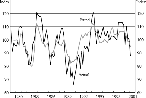
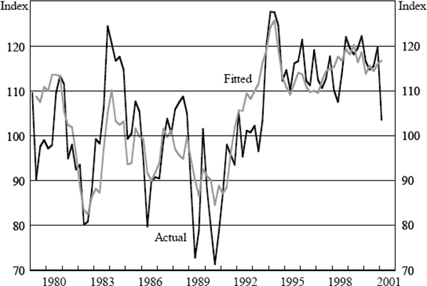
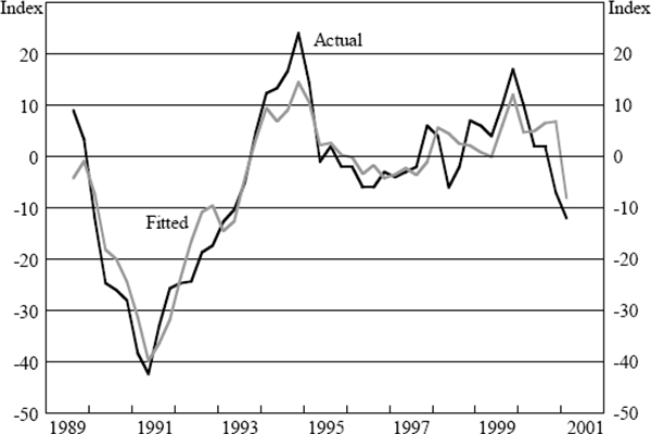
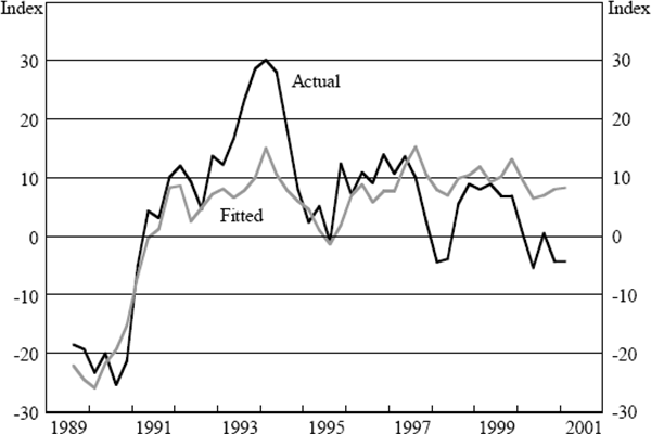
Results for the aggregate indices are presented in Table 1 and Figures 1–4. In this table GDP is gross domestic product, JV is job vacancies (ANZ measure), HW is hours worked, AO is the real All Ordinaries stock index, ER is the A$/US$ exchange rate, and CASH is the official cash rate. The ‘relevant R2’ statistic also needs some explanation. As we are estimating AR(1) models the standard R2 reported by our econometrics package includes the variation explained by the autoregressive component of the errors. However, for the purposes of this exercise we are more interested in the proportion of variation explained by the regressors alone, that is, excluding the unexplained errors even though we have a model for the autoregressive nature of these errors. For this reason we calculate a different R2 statistic, which we call the ‘relevant R2’, by dividing the sum of squares for the fitted series by the standard total sum of squares.[13] The following four figures show the actual and fitted values for these series. In the case of the fitted values we remove the autoregressive error term so that the influence of the underlying variables is clear.
| Regressor | Westpac-MI ICS | Roy Morgan CCR | NAB Business Confidence | NAB Business Conditions |
|---|---|---|---|---|
| ΔGDPt−2 | – | – | – | 2.55 (1.30)* |
| ΔGDPt−3 | – | – | – | 4.15 (1.48)*** |
| ΔGDPt−4 | – | – | – | 4.02 (1.43)*** |
| ΔJVt−1 | 0.28 (0.14)** |
– | 0.29 (0.16*) |
– |
| ΔJVt−2 | 0.47 (0.13)*** |
– | – | – |
| ΔJVt−3 | – | – | −0.39 (0.18)** |
– |
| ΔJVt−4 | −0.26 (0.14)* |
– | −0.62 (0.17)*** |
– |
| ΔHWt−1 | – | – | – | 7.81 (1.92)*** |
| ΔHWt−2 | – | 2.86 (1.62)* |
– | 3.85 (2.25)* |
| ΔAOt−1 | 0.15 (0.09)* |
0.21 (0.09)** |
– | – |
| ΔOt−2 | 0.21 (0.10)** |
0.39 (0.15)** |
||
| ΔAOt−3 | – | 0.27 (0.09) |
0.22 (0.11)* |
0.32 (0.15)** |
| ΔERt | – | 0.29 (0.15)* |
– | – |
| ΔERt−3 | – | −0.39 (0.16)** |
– | – |
| ΔERt−4 | – | – | – | 0.61 (0.24)** |
| CASHt | −1.04 (0.40)** |
−1.07 (0.48)** |
– | – |
| CASHt−1 | – | – | – | −1.20 (0.44)*** |
| CASHt−3 | – | −1.32 (0.48)*** |
−2.77 (0.74)*** |
– |
| Rho | 0.64 (0.09)*** |
0.62 (0.09)*** |
0.82 (0.10)*** |
0.59 (0.18)*** |
| Constant | 10.22 (4.50)** |
21.94 (4.85)*** |
21.40 (7.18)*** |
−4.87 (4.97) |
| Observations | 86 | 87 | 47 | 47 |
| R2 | 0.72 | 0.79 | 0.88 | 0.91 |
| Relevant R2 | 0.39 | 0.69 | 0.67 | 0.72 |
| Q (1–8) p-value | 0.13 | 0.15 | 0.16 | 0.11 |
Note: *, **, *** denote significance at the 10%, 5% and 1% levels. |
||||


Chow tests conducted on the consumer confidence equations provided some suggestion of parameter instability (3 to 4 of 26 potential breakpoints tested returned significant p-values, albeit p-values unadjusted for the sequential nature of our tests). Conversely, CUSUM tests gave no indication of parameter instability. We did not conduct breakpoint tests for the NAB survey measures in view of the short run of data, but CUSUM tests for both measures revealed no evidence of structural instability. We take these results as a broad indication that there are no serious parameter instability problems.
3.3.1 Discussion
The above regressions show that broadly speaking between 40 and 70 per cent of the variation in the sentiment indices we examine can be explained by information that is already available. This argues for a significant backward-looking component to the indices. In all of the regressions the cash rate has a significant influence on the indices and in most of the regressions the last few quarters of hours worked or job vacancies are significant. GDP growth, exchange rate changes and stock market changes also make an appearance in at least one regression. Furthermore, the variable coefficients generally have signs in line with expectations. For example, rises in the cash rate reduce sentiment, falls in the stock market reduce sentiment, and increases in GDP growth improve sentiment.
3.4 Extensions
As foreshadowed above, there are many things one could do differently when analysing sentiment indices. In this section we consider some in an effort to learn more about the information contained in sentiment indices.
3.4.1 Can we improve on the net balance?
The first possibility is that the use of a net balance measure obscures valuable information contained in the distribution of responses.[14] To examine this we looked at the pattern for positive, negative and no change responses for each index separately. On the whole there was little difference between the component series and the net balance series. The proportion of ‘no change’ responses was relatively constant throughout the samples with only minor variation in good or bad times. Regressions using the proportion of positive or negative responses yielded very similar results to those using the net balance on the left hand side. This leads us to the conclusion that there is little to be gained by pursuing this aspect of the data so we confine ourselves to looking at net balance measures throughout the rest of the paper.
3.4.2 Results for individual questions
There is considerable variation in the responses to questions underlying the aggregate indices. Some questions are explicitly backward-looking while others ask about the future. It seems reasonable to assume that the forward-looking questions may provide more information about the future and be less influenced by already available information. To test this and look more closely at the individual components of the surveys we conduct the same exercise for the individual questions as we conducted for the aggregate series. Due to the space taken by the results we report them in Tables B1 to B5 in Appendix B.
In common with regressions for the aggregate indices, serial correlation was present in the residuals. Thus, we again estimated AR(1) models for each equation. Both Chow and CUSUM tests suggest that the first and fifth component indices obtained from the Westpac-Melbourne Institute and Roy Morgan surveys suffer from parameter instability (although the instability seems more pervasive in the case of the fifth). The substitution of alternative specifications did not resolve this problem. Thus, results presented for Indices 1 and 5 should be interpreted with particular caution, and the results for Index 5 might at worst be regarded as uninformative. CUSUM tests for two of the equations for Business Conditions (namely, 12-month Outlook – Expected Profitability and Employment) revealed evidence of structural instability.
3.4.3 Discussion
As far as the two consumer confidence indices are concerned, there seems to be little correlation between the time horizon of the question and the proportion of variation that can be explained by already available economic indicators. The same is true if we compare the components of Actual and Expected Business Conditions (3-month Outlook). This is not really surprising, as the two series show negligible independent variation. The model specifications for the two sets of indices are also very similar. However the Expected Business Conditions (12-month Outlook) regressions display a much poorer average fit to the data than those corresponding to shorter horizon indices. In the next section we address the possibility that the unexplained variation in more forward-looking indices is itself ‘forward looking’ and, for this reason, not readily explained by lagged economic variables.
There is little to be learnt from looking at the set of significant right-hand side variables across equations. The NAB survey indicators and their components are both well explained by a small pool of regressors (comprising both financial and activity variables), which remain relatively constant across horizons, and do not seem specific to the questions asked.[15] Comparing the Roy Morgan and Westpac-Melbourne Institute component index specifications is also uninformative, as the two sets of equations do not closely resemble each other. Perhaps the most striking result is that 61 per cent of the variation in Index 4 of the Roy Morgan survey (economic conditions over the next five years) can be explained solely by lags of the cash rate.
Footnotes
These questions were initially devised by Katona as ‘ice breaker’ questions for the Survey of Income and Wealth in the US (Lovell and Tien 2000). As such they are quite vague and were not specifically designed to give clear answers. This makes the interpretation of this series particularly difficult. [10]
We investigated other alternatives, such as averaging the monthly results, and found that there were no appreciable differences in the regressions. To the extent that there were differences we were generally able to explain the end-quarter observations better. [11]
As might be the case if the survey proved to be a good indicator of current quarter growth and the official release was not made until much later. [12]
We use the de-meaned sentiment series yt as our regressand in each
case (i.e.,  ). Assuming the residuals ut
are autocorrelated (ut =
ρut−1+ εt), the
ordinary R2 will be:
  where
where  To
obtain the ‘relevant R2’, we simply replace
  with
with  thereby removing the effect of the autoregressive
coefficient
  .
[13]
While this possibility has received scant attention in the literature, at least one research effort has used the proportion of ‘no answer’ and ‘don't know’ responses to a business survey as a predictor in forecasting regressions, apparently with significant results (Dunkelberg and Dennis 1988). [14]
The exception is that GDP growth does not predict Business Conditions 12 months ahead, but it is hard to make much of this result. [15]