RDP 2002-01: Inflation Targeting and the Inflation Process: Some Lessons from an Open Economy 3. Evidence from a Small Empirical Macro Model

The discussion in the previous section implies that the choice of the appropriate inflation target is, in large part, an empirical issue that depends on the structure of the economy and the specification of the welfare function. In this section, we use a small model of the Australian economy to illustrate the trade-off curves and their sensitivity to the structure of the economy. On the basis of these, some conclusions can be drawn on the relative merits of targeting aggregate and non-traded inflation.

This extends the work of Bharucha and Kent (1998) who examined the choice of inflation target in a simple calibrated version of the Ball and Svensson model, and focused in detail on the influence of different shocks on this choice. Ryan and Thompson (2000) also examined the issue using a model of the Australian economy, in terms of simple policy rules. The analysis here focuses primarily on optimal policy, although some policy rules are considered to provide a basis of comparison with Ryan and Thompson.

3.1 Methodology

The trade-off curves are generated using a simple empirical model of the Australian economy similar to that in Beechey et al (2000).^[3] The model is a more complex version of the simple Ball-Svensson framework discussed in Section 3, but the central features are the same, namely an equation for output, aggregate inflation, and an objective function for the central bank.^[4]

As in the Ball-Svensson model, there are two channels of transmission of monetary policy to output: directly through changes in the real interest rate (with a six-quarter lag) and indirectly through changes in the real exchange rate (with a four-quarter lag). The real exchange rate is explained by movements in the terms of trade and real interest rate differentials.

Aggregate inflation is measured by changes in the consumer price index. It depends on contemporaneous and lagged changes in import prices, lagged growth in unit labour costs and its own lags (proxying backward-looking expectations). There is no forward-looking component of inflation expectations.^[5] The majority of the effect of exchange rate changes on import prices is assumed to occur contemporaneously, consistent with estimates of first-stage pass-through (Dwyer, Kent and Pease 1994). Hence exchange rate changes are transmitted immediately to aggregate inflation (although the initial impact is relatively small). Monetary policy affects aggregate inflation through its impact on the output gap in the unit labour cost equation and through its effect on import prices via the exchange rate.

As an appropriate specification of inflation in the central bank's reaction function in an open economy, Ball (2000) advocated a measure of long-run inflation that filtered out the transitory effects of exchange rate fluctuations. Initially, we tried a measure of inflation based on the prices of non-traded goods in the consumer price index. However, this proved to be dependent on exchange rate fluctuations, because of the importance of imported inputs in the production of non-traded goods, and also of government-determined prices.^[6] Instead we use unit labour costs as a measure of inflation in the non-traded sector (hereafter unit labour costs and non-traded inflation are used interchangeably). Unit labour costs are modelled using a Phillips curve specification, with expectations modelled as a weighted average of aggregate and non-traded inflation. Hence, while there is no direct effect of the exchange rate on unit labour costs, there are indirect effects through the influence on inflation expectations and the output gap.

The policy-maker is assumed to have an objective function as described in Equation (4). Two forms of the objective function are considered: one with aggregate inflation, the other with growth in unit labour costs. To generate the trade-off curves, the relative weight on output variability (λ) is varied between 0 and 1. The instrument of monetary policy is the nominal cash rate.

The model of the economy is then simulated by taking draws of the error terms in each equation for both exogenous and endogenous variables, using a distribution based on the estimated variance-covariance matrix. The policy-maker is assumed to know the full structure of the economy but assumes the value of all future shocks is zero. Each period the policy-maker chooses the optimal level and future path for interest rates to minimise the objective function. The model was simulated for 100 periods for each value of λ, and the variability of output, aggregate and non-traded inflation was calculated in each simulation.

3.2 Results

3.2.1 Optimal policy

The top panel of Figure 1 shows the trade-offs between output variability and aggregate inflation variability when aggregate inflation is the objective and when non-traded inflation is the objective. Similarly, the bottom panel shows the trade-off between output variability and non-traded inflation variability for the two different objective functions. As a point of comparison, the actual historical outcomes are also shown (for the period 1985:Q1–1999:Q4).

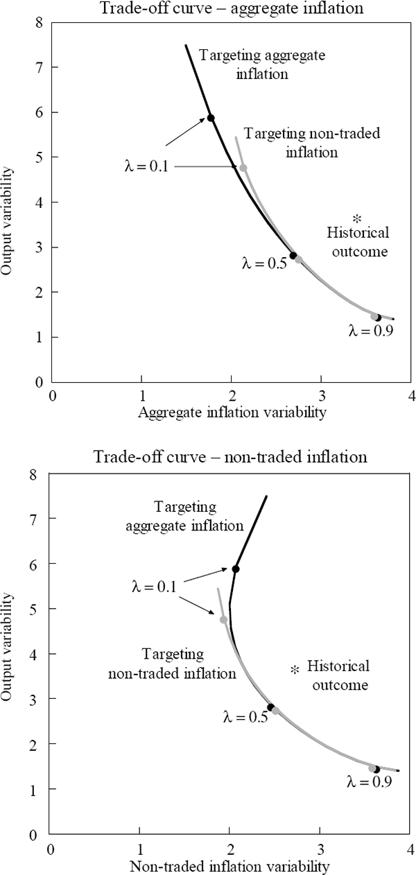
The figure illustrates the obvious conclusion that the best way to minimise the variability of a particular measure of inflation is to directly ‘target’ that measure, by placing it in the objective function. The upper panel shows that the variability of aggregate inflation is not significantly higher when non-traded inflation is targeted. A small difference only emerges as relatively more weight is placed on inflation variability (as λ declines). This result is not surprising because aggregate inflation is an important determinant of non-traded inflation. Therefore, in minimising the variability in non-traded inflation, the policy-maker will also seek to reduce the variability in aggregate inflation.

The converse is also generally true except when there is a relatively large weight on inflation variability (when λ is less than about 0.25). In those circumstances, strict inflation targeting generates considerably more variability in non-traded inflation. Consequently, those parts of the economy for which non-traded inflation is more important will be worse off under a strict aggregate-inflation targeting regime.

When a strict aggregate inflation target is pursued, output variability is also considerably higher than under a strict non-traded inflation target. These results are similar to those in Svensson (1998), who also finds that strict inflation-targeting regimes generate a large amount of volatility in ‘domestic’ inflation and output.

In these simulations, the policy-maker is able to exactly distinguish between temporary and permanent shocks to the exchange rate and respond appropriately. In practice, this is considerably more difficult. These results suggest that there may not be much cost in focusing on a non-traded measure of inflation. That is, the policy-maker need only respond to the exchange rate changes to the extent that s/he expects them to be reflected in movements in non-traded inflation.

The variability of interest rates associated with these trade-off curves is considerably larger than that observed in practice. The standard deviation of the quarterly interest rate changes ranges between 2½ and 5½ per cent per annum. Consequently, the objective function was amended in the normal way to include an interest-rate smoothing term penalising interest rate variability. A weight on the smoothing term that was sufficient to reduce the volatility in interest rates to that observed historically did not have a significant impact on the trade-off curves: the variability in output and aggregate inflation only increased marginally. This result is similar to that in Lowe and Ellis (1997), who also found that reducing the volatility of policy interest rates does not greatly affect the variability of the other target variables. However, when a smoothing objective is included, the increase in the variability of non-traded inflation when a strict aggregate inflation target is pursued is even greater.

To test the sensitivity of these results to the structure of the economy, the model was altered in a number of ways. First, the variability of the exchange rate shocks was doubled.^[7] This naturally shifted the variability frontiers up and to the right but did not materially alter the conclusion that the choice of inflation target does not have much impact except in the case of strict inflation targeting.

Second, the process for the real exchange rate was changed. In the model, long-run movements in the real exchange rate are driven by the terms of trade, which are assumed to be stationary. The terms of trade was changed to a non-stationary process, allowing for permanent shifts in the real, and hence nominal, exchange rate.^[8] The effect of this was to steepen the trade-off curves. That is, increasing the weight on output in the objective function led to a larger reduction in output variability and a smaller increase in inflation variability than the baseline case. However, again, there was very little difference in outcomes for the two different inflation objectives.

Third, the expectations process in the non-traded sector (unit labour costs) was altered to allow for some credibility in the inflation target. A positive weight was placed on a constant term set equal to the inflation target, thereby anchoring unit labour costs in the long run. However, inflation expectations retained some backward-looking element. This change to the expectations process naturally shifted the trade-off curves towards the origin, as the expectations process was less volatile. That is, establishing credibility in the inflation target allows the policy-maker to choose from a superior set of economic outcomes. The choice of inflation target did not result in any significant differences in the variability of either measure of inflation. However, a strict aggregate inflation target generated even more variability in output compared to a strict non-traded inflation target, than in the baseline case.

3.2.2 Policy rules

To date, the analysis has been conducted in terms of optimal policy. Ball (1998), Svensson (1998) and Ryan and Thompson (2000) all examined the choice of the appropriate inflation target in the context of Taylor-type policy rules. In the simple Ball-Svensson framework, a Taylor rule that includes the exchange rate is the optimal policy reaction function. However, in more complicated models like that used in this section, such rules may only be rough approximations to optimal policy. Optimal policy in these models takes account of changes in all the variables in the economy, rather than only the variables in the policy rule. The simple rules, however, may be useful to the extent that aggregate output and inflation are summary statistics for developments in the economy, or that tractable and transparent rules are desirable.

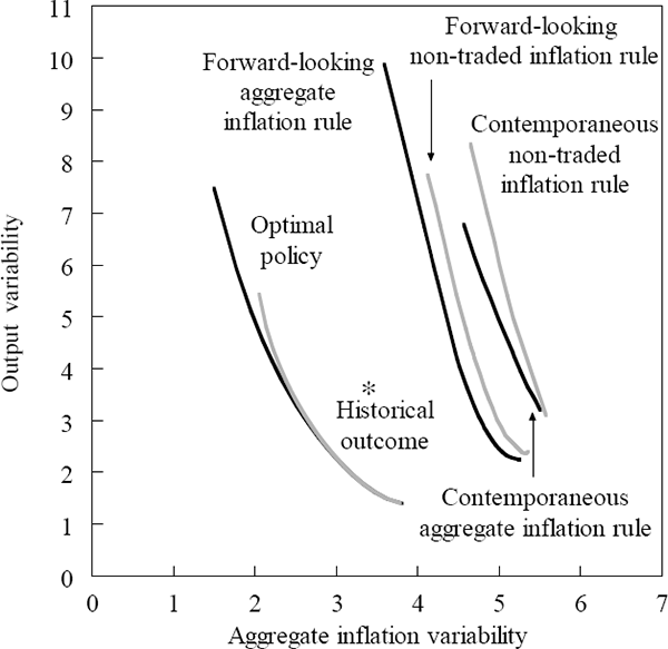
To investigate the trade-off when the central bank follows a policy rule, the model was simulated in the same way as in the previous section except that the central bank follows a rule rather than optimising an objective function every period. Two policy rules were examined: one with weights on output and aggregate inflation, the other with weights on output and non-traded inflation. In the first set of simulations, these policy rules were contemporaneous, including only current-dated measures of inflation and output. Simulations were then conducted using forward-looking rules, where the forecast of output and inflation three quarters ahead entered the policy rule.^[9] In each case, a number of simulations were conducted for different sets of weights on output and inflation in the policy rule. An efficient frontier for each rule traces out the lowest combinations of inflation and output variability as these weights are varied.

Figure 2 shows the efficient frontiers from rules that respond to contemporaneous movements in output and aggregate inflation and rules that respond to forecasts for these variables. By way of comparison, it also shows the optimal policy frontiers derived earlier. The frontiers for the policy rules result in significantly more variability in inflation and output than optimal policy, and indeed than that which was actually observed in practice. These simulations also confirm two results in Ryan and Thompson (2000). Firstly, an aggregate inflation rule generates a more preferable trade-off than a non-traded inflation rule, although the differences between the two rules are not stark. Secondly, a forward-looking rule leads to lower output and inflation volatility than a contemporaneous rule.

3.2.3 Summary

The results of these simulations suggest that in a representative model of the Australian economy, targeting aggregate inflation and targeting non-traded inflation deliver similar economic outcomes. This occurs because exchange rate changes have a muted effect on aggregate inflation. The only exception to this conclusion is that a strict aggregate inflation target significantly increases the variability of non-traded inflation and output, as greater reliance is placed on the faster-acting exchange rate channel of monetary transmission.

As mentioned earlier, an important caveat to this conclusion is that the simulations assume the policy-maker is able to distinguish between temporary and permanent movements in the exchange rate. These results are also very sensitive to the nature of the inflation process. The next section examines how this has changed over the past two decades.

Footnotes

The model is described in detail in Appendix A. Beechey et al (2000) also provides a summary of macroeconomic developments in the Australian economy over the past two decades, and further details are provided in Gruen and Shrestha (2000). [3]

We assume the central bank doesn't discount outcomes in future periods, i.e. in Equation (4) θ is assumed to be unity throughout the simulations. [4]

Backward-looking expectations have historically been an accurate characterisation of the inflation expectations process of households in Australia (Brischetto and de Brouwer 1999). Beechey et al (2000) find a role for a measure of inflation expectations obtained from the bond market. [5]

Ryan and Thompson (2000) also found that non-traded inflation was sensitive to exchange rate movements, and examined a policy rule that targeted unit labour costs in the non-traded sector. [6]

It was assumed that this change in the variability did not alter any other aspect of the model. [7]

This also implies a permanent shift in the neutral real interest rate. [8]

Ryan and Thompson (2000) present results which suggest that three quarters is the most efficient horizon for a Taylor rule in a model similar to that used here. [9]