RDP 2002-08: Currency Crises and Macroeconomic Performance 3. The Model
November 2002
- Download the Paper 136KB
3.1 The Basic Model
This section presents a familiar monetary model which rationalises some of the stylised facts about currency crises that were presented in Section 2. It is a simple variation on the framework proposed by Buiter and Miller (1982), consisting of an LM curve, a Phillips curve, an uncovered interest parity condition, and an IS curve. In steady state, domestic prices rise at the same rate as the nominal money supply: goods prices are sticky; the nominal exchange rate moves discontinuously in response to news;[7] the monetary authority controls the rate of nominal money supply growth; and market expectations of all endogenous variables are rational. The income variable has a steady state value of zero, and so lends itself to interpretation as a measure of the output gap.
Formally, the model's behavioural equations are:
where:
m = (natural logarithm of) the nominal money stock;
p = (natural logarithm of) the domestic price level;
l = (natural logarithm of) real money balances;
e = (natural logarithm of) the home-currency price of a unit of foreign currency;
c = (natural logarithm of) the real exchange rate;
y = the output gap;
r = the domestic nominal bond yield;
r* = the foreign nominal and real bond yield (exogenous);
rd = the rate of interest on domestic money holdings (exogenous); and
 (exogenous).
These equations are standard in all but two respects. First, the opportunity cost of real balances is given, not by the lending rate of interest, but by the difference between that rate and the deposit rate of interest, rd. Although this was a feature of the original Buiter-Miller model, its implications were not explored at length. It will feature prominently in the dynamics described below.
A more genuine innovation is our modelling of inflation. In the original Buiter-Miller model, inflation depends exclusively on the output gap and the rate of money supply growth. So, for fixed money supply growth, a nominal exchange rate depreciation only boosts inflation because it also stimulates competitiveness and output, thus leading to a movement along the short-run Phillips curve.
Section 2 suggests that this transmission mechanism does not describe currency crises very well, since prices often rise after sudden depreciations, even though output may actually fall. The missing element may be the import price inflation that follows a sudden depreciation, since this will not necessarily be related to output. To capture this, we have assumed that the inflation process is related not only to money supply growth and the output gap, but also to the difference between the real exchange rate and its equilibrium level; that is, c(t) − γr*/δ.[8] In a dynamically stable economy, this aspect of the inflationary process will only be temporary. As the real exchange rate converges on its equilibrium level, the shock to import prices subsides.
It seems unlikely that inflation associated with import price pass-through would feed through into lower real domestic interest rates. Indeed, as the Asian crisis of the late 1990s demonstrates, non-financial corporations typically face sharply higher borrowing costs after sudden depreciations, especially if they have unhedged liabilities in foreign currency. We capture this rise in the real interest rate by modifying the IS equation (Equation (6)), and choosing a value of φ which is greater than one. Although this adjustment is ad hoc, it overcomes the otherwise implausible prediction of the model that economic activity will necessarily rise as a result of the rise in inflation that accompanies a currency crisis.
We consider two alternative sets of shocks to the model: a simple currency crisis, and a twin crisis. A simple crisis happens when the world interest rate rises suddenly and unexpectedly, forcing a sharp depreciation. A twin crisis follows when the rise in world interest rates and the shock to the currency force banks to stem bank runs by raising the deposit rate, rd.
Equations (3) through (8) collapse into the following system of equations:
where:
This system is saddlepoint stable if its two characteristic roots are real and of opposite sign. For present purposes, this is a necessary property, since only a saddlepoint implies the discontinuous jumps in the nominal and real exchange rates which characterise currency crises. The condition which gives this saddlepoint stability, and which we assume to hold, is:
A sudden depreciation of the currency is most easily, and plausibly, generated with an unexpected rise in the world interest rate. This seems to have precipitated, or at least preceded, a number of crises in recent history. The ERM crisis of 1992 and some of the Latin American crises of the 1980s are good examples. For present purposes, we will assume the increase in the world interest rate to be unanticipated and permanent.
To simulate the banking crises that sometimes coincide with currency crises, consider the possibility of a rise in the domestic deposit rate.[9] This takes the deposit rate above the lending rate and it is both unanticipated and contemporaneous with the rise in the world interest rate. It has the effect of making some real balances unavailable for use in either consumption or investment. Of the several rationalisations that could support this assumption, we favour the possibility that the rise in world interest rates has caused some distress among domestic banks and forced them to raise rates on their liabilities in a bid to stem a bank run.
If the banking system is inter-temporally solvent, the deposit rate cannot permanently exceed the lending rate. Assume, therefore, that the deposit rate increase is of finite but uncertain duration. Specifically, the banking crisis is assumed to begin at t = 0, and end at a date T, determined stochastically as the outcome of a Poisson process with rate ε.
As should be clear, the endogenous variables in the model evolve over time along deterministic paths. With the arrival of any shock, there will be shifts in these deterministic paths at the time of the shock and out into the future. In the case of a banking crisis, the only uncertainty in the model once the crisis has begun arises from the assumed stochastic nature of the end of the crisis. When the crisis does end, the time-paths of the endogenous variables will shift.
We therefore introduce the notation that, for the endogenous variable x, x(t) follows the deterministic path f(t) while the banking crisis is occurring, for t < T, and the path g(t,T) after the crisis has ended, t≥T.
Rather than calculating the details of these deterministic paths, we focus instead on the expected value of the endogenous variables formed at the beginning of the crisis at t = 0, E0[x(t)], and examine how this expectation evolves over time (as t rises). To calculate E0[x(t)], we integrate over the uncertain end-date of the crisis, T:
The analytical solutions for the expected paths are unsightly, and they are best explained with the aid of some simple simulations. Table 11 reports a set of parameter estimates for this exercise. Although the parameters seem reasonable to us, they have been chosen more or less arbitrarily, with the satisfaction of stability conditions in mind. Only two further comments on them seem necessary. First, the parameter φ has been set at a reasonably high level, since at lower levels the exchange rate may not overshoot, and at much higher levels, saddlepoint stability is threatened. Second, the calibration of the model gives the banking crisis an expected duration of five years.
| Parameter | Value |
|---|---|
| κ | 1.0 |
| λ | 0.3 |
| ϕ | 0.1 |
| α | 0.5 and 0.0 |
| δ | 0.2 |
| φ | 3.0 |
| γ | 0.8 |
| μ | 0 |
| ε | 0.2 |
| dr* | 0.050 (500 basis points) |
| drd | 0.075 (750 basis points) and 0.0 |
Figures 2 to 5 report four sets of simulation results. Figures 2 and 4 show the dynamic behaviour of the economy when there are twin banking and currency crises, while Figures 3 and 5 show the dynamics when there is no banking crisis and hence rd is unchanged. Figures 2 and 3 show the case in which the import price effect is operative, while Figures 4 and 5 show the results from the more standard case. All results report deviations of the variables from a common baseline of zero.
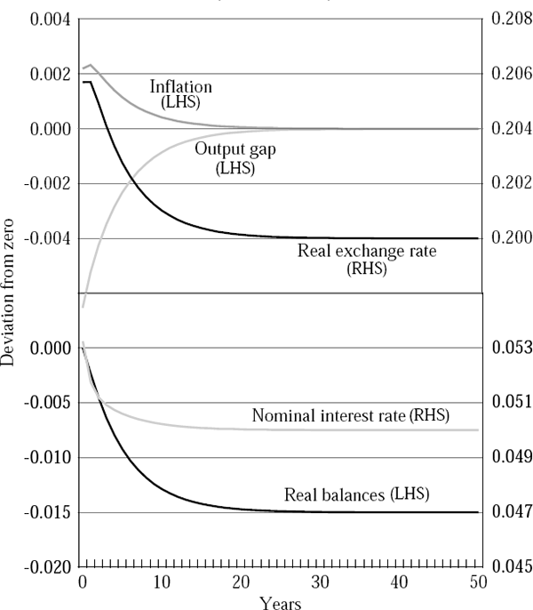
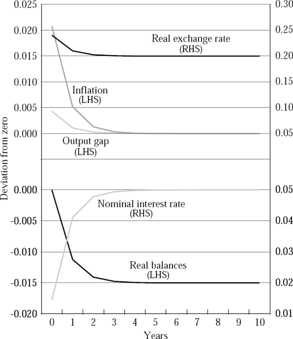
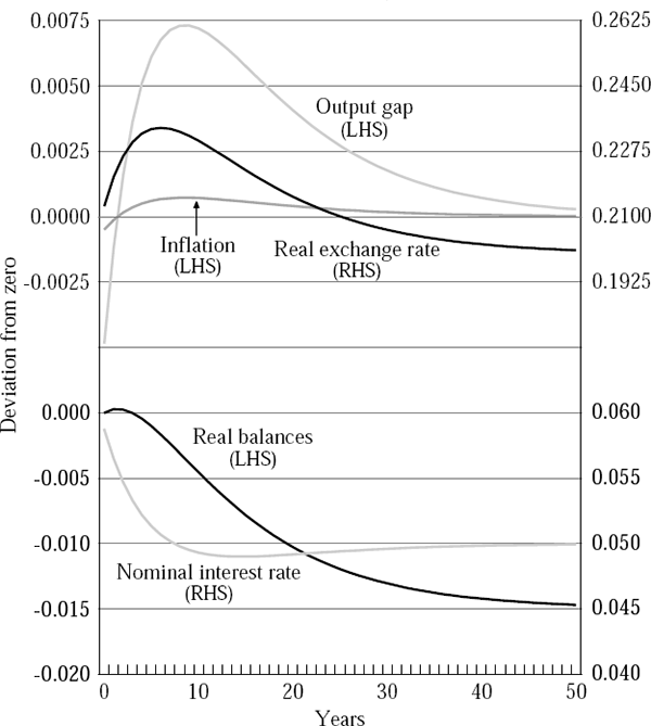
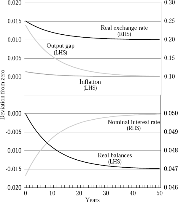
A key result is that while the nominal exchange rate depreciates in both cases, output only falls when there is a twin crisis.[10] A simple increase in the world interest rate is expansionary, because it causes the nominal exchange rate to depreciate in the short run. However, if there is a banking crisis and the deposit rate of interest rises, liquidity will be withdrawn from the system and the nominal borrowing rate of interest will rise sharply. The simulations show that the contractionary effects of this rise can outweigh the stimulus from the exchange rate. The inflation outcomes also depend on whether there are simultaneous banking and currency crises, but only if there is an import price channel at work.
Figures 2 and 3 show that inflation will rise after a shock and that a banking crisis will influence the extent of that rise. Figures 4 and 5 show simulations with no import price pass-through, and the outcomes are different. Currency crisis simulations show the deterministic path of variables after the crisis. Twin crisis simulations show the expectation of the variables' paths formed immediately after the crisis (at t = 0). In these simulations, the response of inflation is very modest, irrespective of whether or not there has been a banking crisis.
3.2 Optimal Policy
After the east Asian currency crisis, there was much debate about the best monetary policy response to shocks which induce simultaneous depreciations and output contractions. Some have argued that depreciation should not be resisted in these circumstances because tighter monetary policy would probably be self-defeating (Furman and Stiglitz 1998; Stiglitz 1998). Higher interest rates may undermine the banking system and perhaps weaken confidence in the economy to the point of perpetuating, rather than easing, the depreciation to which they were addressed. Moreover, tighter policy may not be credible in the face of falling output, in which case financial markets will certainly discount or ignore it. Kraay (2000) documents some general evidence against the effectiveness of tighter policy, showing a striking lack of correlation between interest rate settings and the outcome of speculative attacks.
The more traditional position, as stated by Fischer (1998), is that the damaging effects of depreciation on confidence and financial stability can only be arrested if the costs of short-selling the currency are raised quickly and sufficiently; that is, if monetary policy is tightened. To this, Goldfajn and Gupta (1999) add that inflation is a consideration when setting policy in the wake of a crisis. They argue that central banks should prefer to see a disequilibrium real depreciation corrected with nominal appreciation, rather than inflation. And their evidence suggests that, unless the currency crisis coincides with a banking crisis, a nominal appreciation is often achieved with tighter monetary policy.
Our model offers a formal framework which engages both the orthodox and the alternative perspectives. Assume that the rate of money growth is set by a monetary authority which takes as given the structure of the economy and the shocks to r* and rd. Faced with these shocks, it implements the change in the money growth rate which minimises a loss function that punishes output gaps and non-zero inflation. For the sake of simplicity, this adjustment to the money growth rate is assumed to be once-off and permanent. The problem then reduces to:
where:
where ν and θ are preference parameters describing the discount rate and the weight that the monetary authority places on output deviations.
To solve this problem, remove the expected rate of inflation using the Phillips curve. Then assume that any change to the monetary policy rule which the shock might induce is contemporaneous with, and as unanticipated as, the changes in the two exogenous interest rates. Speculators are assumed to treat the policy change as credible and permanent, since it represents a solution to a well-defined social welfare problem. Consistency between the policy itself and market expectations of it makes both private and public behaviour optimal.
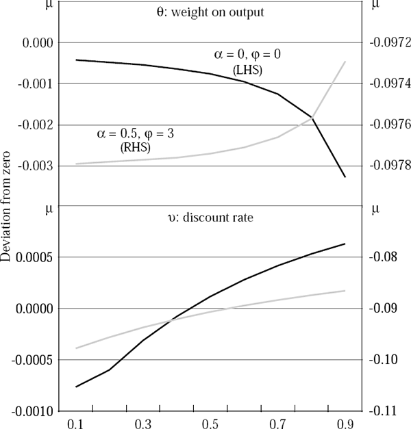
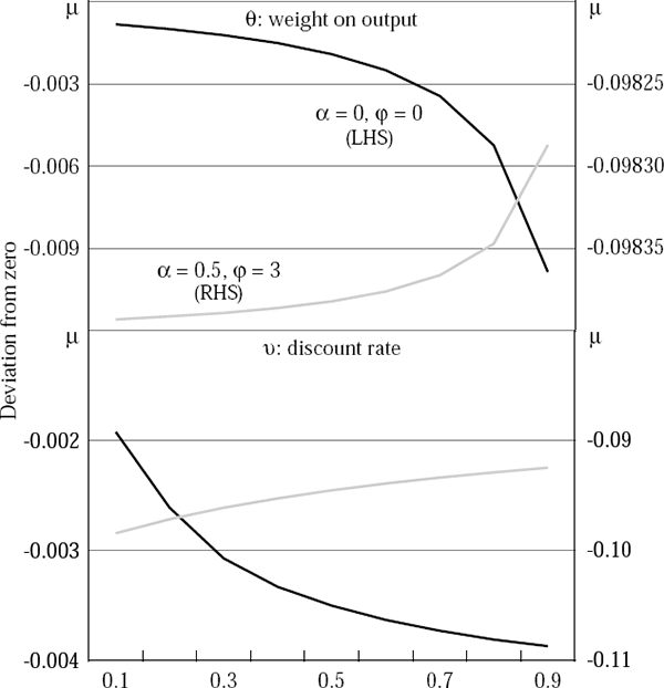
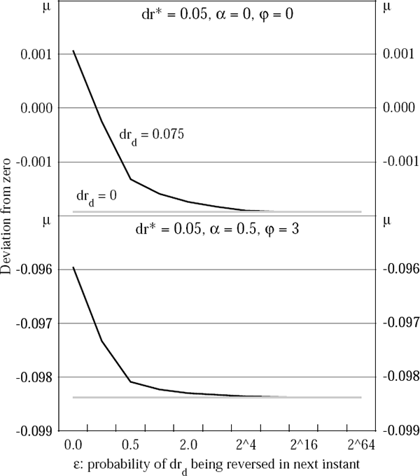
Figures 6 through 8 show the optimal policy response (that is, the optimal choice of the money growth rate, μ) to currency and twin crises, using the parameter values in Table 11. The effects of varying θ, ν and ε on the optimal choice of μ are highlighted. In most cases, it is optimal to tighten in response to either set of shocks. However, if the monetary authority has a high discount rate, or if the banking crisis threatens to be very protracted, then the present value of lost output is high and so it can be optimal to increase the money growth rate, that is, to ease monetary policy.
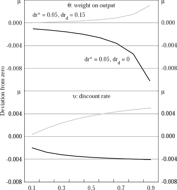
A final set of simulations highlights the sensitivity of these policy prescriptions to the differentials between the exogenous interest rates and to import price inflation. The twin crisis case assumes a 1,500 basis point increase in rd and no direct import price inflation. The simple currency crisis case assumes a 500 basis point increase in r*.
The optimal policies for these cases are profiled in Figure 9. They show that monetary policy depends quite heavily on the behaviour of the banking system – an easing is likely to be appropriate during a twin crisis, but unwarranted when only the world interest rate rises. In the twin crisis case, the opening of a large differential between the two domestic interest rates tends to push output down heavily, while a subdued inflation response removes any incentive which the monetary authority may otherwise have had to tighten.
These final results accord reasonably well with the conclusions of Aghion, Bacchetta and Banerjee (2000). Using a model which is simpler than, but broadly similar to, ours, Aghion et al find that it may well be optimal to ease policy when the financial system is distressed by the crisis, and when the proportion of foreign currency denominated corporate debt is high.
Footnotes
The fact that the nominal exchange rate moves between steady states does not preclude the possibility that it could have been fixed in the initial steady state. [7]
The term γr*/δ is the equilibrium real exchange rate, for any values of α or φ. [8]
We do not model the actual transmission of the currency crisis to the banking crisis. [9]
Since prices are sticky, initial movements in the nominal exchange rate are identical to the movements in the real rate. [10]


