RDP 2003-11: How Should Monetary Policy Respond to Asset-Price Bubbles? 3. Results
November 2003
- Download the Paper 192KB
In this section, we present optimal policy recommendations through time, assuming that the bubble survives and grows. We focus on the growth phase of the bubble's life because it is of most policy interest, as it generates the most disagreement about which policy approach is preferable. Once the bubble bursts, by contrast, there is general agreement that it is appropriate to ease aggressively to offset the contractionary effects of the bust.[5]
Our main aim is to compare the optimal policy recommendations of the sceptic with those of an activist, over a range of plausible alternative assumptions about the stochastic nature of the bubble. To do so in a meaningful way, it is necessary that the two policy-makers face an economy in the same state in each year. Since the current state of the economy depends on previous policy settings (as well as on the evolution of the bubble) we will assume throughout that the policy settings that are actually implemented each year are those chosen by the sceptic.
We can then meaningfully ask each year: given the state of the economy, what are the current optimal policy recommendations made by the different policy-makers? The activist's recommendations will depend on the assumptions she makes about the future possible paths of the bubble, while the sceptic's will not, since she assumes that future asset-price shocks have no expected effects.
3.1 Baseline Results: Policy Cannot Affect the Bubble
We begin with some simple baseline results. For these results, we assume that the bubble's direct expansionary effect on output in each year of its growth is a constant 1 per cent (i.e., γt = 1). Figure 1 shows the optimal policy choices made by the sceptic and two activists. We focus first on the sceptic, and then on the activists.
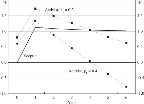
Notes: The sceptic implements policy in each year. Real interest rates are deviations from neutral.
Since the sceptic assumes that future asset-price shocks have no expected effects, she responds to the bubble only when its initial expansionary effects are manifest in year 1. As time proceeds and the bubble grows, she sets the policy interest rate in line with Equation (7), which is optimal given her beliefs about future asset-price shocks. Of course, were the bubble to burst, she would ease immediately (see Appendix A for further details).
An activist, deciding on optimal policy in year t, understands that if the bubble continues to grow, its direct effect on output next year will be +1 per cent, while if it bursts, the direct effect next year will be −αt per cent. If the probability of bursting each year is a constant, p*, the bubble's expected direct effect on output next year is (1 − p*) − p*αt.
Certainty equivalence applies to this baseline version of the model.[6] It follows that
the difference between the policy interest rates recommended by the activist,  , and the
sceptic,
  ,
depends only on their different assessments of the expected effect of the bubble on output next
year. With the sceptic assuming that the bubble will have no expected effect on output next
year, it follows that
Equation (8) implies that the activist will recommend tighter (easier) policy than the sceptic whenever, in probability-weighted terms, the expansionary effect on real activity from the bubble surviving is greater (less) than the contractionary effect from the bubble collapsing.
For the results shown in Figure 1, we assume that the only difference between the two activists is that one assesses the probability that the bubble will burst each year as pt = p* = 0.2 (the ‘durable-bubble activist’), while the other assesses it as pt = p* = 0.4 (the ‘transient-bubble activist’).[7]
In terms of their optimal policy recommendations, the two activists agree that policy should be tighter than the settings chosen by the sceptic for the first couple of years of the bubble's growth (including year 0, since that is when they learn about the bubble). Although they disagree about the details, they share the assessment that the continued probable growth of the bubble is a more important consideration for policy than the bubble's possible collapse.
The activists both understand, however, that as time proceeds, the bubble is getting bigger and the size of the prospective bust is also getting bigger. As a consequence, if the bubble survives for more than a year or two, the two activists no longer agree about whether policy should be tighter or looser than the modified Taylor-rule settings chosen by the sceptic. The durable-bubble activist recommends tighter policy because she assesses the probability of the bubble bursting to be small, but the transient-bubble activist recommends looser policy because her assessment is that this probability is larger.
If the bubble survives for long enough the two activists will again concur at least in the direction of their policy advice – they will both recommend looser policy than the sceptic because the possibility of the by-now-bigger bubble collapsing eventually dominates for them both.
In this case, then, the policy recommendations of an activist – and even whether she recommends tighter or looser policy than the benchmark settings chosen by the sceptic – depend crucially on her assessment of the probability that the bubble will collapse of its own accord. This is an important example of the general point that the activist's policy advice will depend critically on the detailed assumptions she makes about the stochastic properties of the bubble. This is the central insight of the paper. We now show the relevance of this insight across a wide range of alternative assumptions about the bubble's stochastic behaviour.
3.2 Sensitivity Analysis[8]
3.2.1 Policy affects the probability that the bubble will burst
An obvious extension to the model is to assume that by setting tighter policy this year, the policy-maker can raise the probability that the bubble will burst next year. For simplicity, we initially assume a linear relationship between the interest rate and the probability of the bubble bursting:
We assume that δ = 0.1, so that a 1 percentage point rise in the real interest
rate this year raises the probability of the bubble bursting next year by 0.1, subject to the
constraint that 0 ≤ pt ≤ 1. The path of interest rates,  , is the
optimal path chosen by the sceptical policy-maker.[9]
As before, we assume that the bubble's direct expansionary effect on output in each year of its growth is a constant 1 per cent (i.e., γt = 1). Figure 2 shows the optimal policy recommendations made by the sceptic and two activists. The two activists again differ only in their assessment of the bubble's probability of collapse. Both believe that this probability is given by Equation (9), but the durable-bubble activist believes that p* = 0.2, while the transient-bubble activist believes that p* = 0.4.
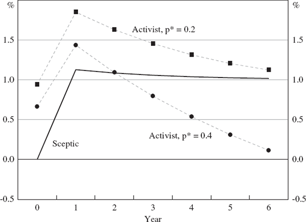
Notes: The probability of the bubble bursting is given by Equation (9) with δ = 0.1. The sceptic implements policy in each year. Real interest rates are deviations from neutral.
The sceptic's optimal policy profile is the same as in Figure 1, because she ignores the future stochastic details of the bubble. By contrast, it is optimal for the activists to recommend tighter policy than they would recommend if they had no influence on the bubble, as can be seen by comparing the activist profiles in Figures 1 and 2. By tightening somewhat, the activists reduce the probability that the bubble will grow further and be more disruptive to the economy when it ultimately bursts. Nevertheless, the optimal policy continues to depend, sensitively, on the activist's assessment of the bubble's probability of collapse, just as it did when the activists could not affect the bubble.
It is also of interest to see how the results change when we vary the sensitivity to interest rates of the bubble's probability of collapse. For this exercise, we assume a monotonically increasing, but non-linear, relationship between interest rates and this probability, to avoid a corner-solution problem with the linear form (explained shortly). The relationship we assume is
where α = −δ/(p*(l − p*)) and
b = ln((1 − p*)/p*). For this functional form,
Pt = P* when  and
and  when this
derivative is evaluated at
  . These two features are also features of
the linear form, Equation (9). The advantage of the non-linear form, Equation (10), is that,
while raising last year's interest rate, rt−1, raises the
probability that the bubble will burst this year, pt, it cannot drive that
probability to one, as can occur with the linear form.[10]
Figure 3 shows a comparison of optimal interest rate recommendations for the sceptic and three activists. The activists assume that the bubble's probability of bursting is given by Equation (10) with p* = 0.4 (except p14 = 1), but they assume three different degrees of interest-rate sensitivity: δ = 0.1, δ = 0.2 or δ = 0.3.
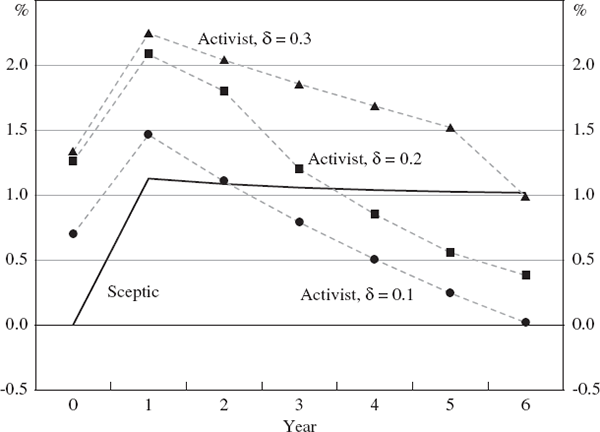
Notes: The probability of the bubble bursting is given by Equation (10) with p* =0.4. The sceptic implements policy in each year. Real interest rates are deviations from neutral.
The pattern of optimal interest rate recommendations is somewhat similar to those in Figures 1 and 2. When the bubble is very small, the activists all agree that policy should be tighter than the setting chosen by the sceptic. But this consensus among the activists evaporates as the bubble gets bigger, and from year 2 onward, first one and then two of the three activists recommend looser policy than the sceptic, while the activist who believes that the bubble is highly interest sensitive (δ = 0.3) continues to recommend tighter policy, at least until year 6.
3.2.2 Allowing for efficiency losses
A second natural extension is to allow for efficiency losses associated with the bubble. There are two broad ways to motivate the idea of efficiency losses. They can be motivated in terms of the economically inefficient physical over-investment that is put in place in response to asset-price rises that are not based on fundamentals, or in terms of the damage done to the financial system when the bubble bursts.
Either way, it seems plausible that the efficiency losses rise with the size of the bubble. To account for these losses, we re-formulate the policy problem as setting rt to minimise
where we assume that the efficiency losses rise either linearly with the maximum size of the
bubble (κ = 1) or with the square of this maximum size (quadratic case,
κ = 2). We also assume, as before, that the relative weight on inflation
deviations, µ, takes a value of one. Since the sceptic ignores the bubble, we
assume for her 
Figure 4 shows a comparison of optimal interest rate settings for the sceptic and three activists. The activists all assume that the bubble's probability of bursting is given by Equation (10) with p* = 0.4, and with interest-rate sensitivity, δ = 0.2. The first activist, however, makes no allowance for efficiency losses, and hence minimises the standard loss function, Equation (6). The second activist assumes linear efficiency losses, while the third assumes quadratic losses, and so they minimise the loss function, Equation (11), assuming appropriate values for κ.
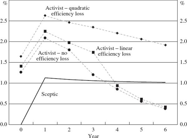
Notes: The probability of the bubble bursting is given by Equation (10) with p* =0.4 and δ =0.2. The sceptic implements policy in each year. Real interest rates are deviations from neutral.
As previous figures have shown, being able to raise the probability of the bubble bursting gives an incentive to the activist policy-maker to tighten policy somewhat. Figure 4 shows that taking account of efficiency losses associated with an asset-price bubble raises this incentive further, and therefore further raises the optimal interest rate recommendations of the activist. Moreover, if efficiency losses associated with the bubble are assumed to rise sufficiently rapidly with the maximum size of the bubble, then the incentive for the activist to recommend tighter policy than the sceptic is a strong one.
3.2.3 Policy affects the bubble's growth
A further natural extension to the simple version of the model involves assuming that, rather than affecting the probability of the bubble bursting, the activist policy-maker can, by setting tighter policy this year, reduce the extent of the bubble's growth next year if it survives. For the simulations we show for this case, we assume that pt = p* = 0.4 (except p14 = 1) and that
For reasons we discuss shortly, only large values of the parameter ϕ generate
significantly changed behaviour by the activist policy-maker. We therefore assume that (
ϕ = 1, so that by setting policy 1 percentage point higher than the sceptic this year,
the bubble's growth next year is reduced from 1 per cent to nothing.[11]
As above, the path of interest rates defined by  , is the optimal
path chosen by the sceptical policy-maker assuming γt = 1.
Figure 5 shows a comparison of optimal interest rate recommendations for the sceptic and two activists. Both activists assume that the bubble's growth is given by Equation (12), but one assumes no interest-rate sensitivity, ϕ = 0, while the other assumes high sensitivity, ϕ = 1.[12]
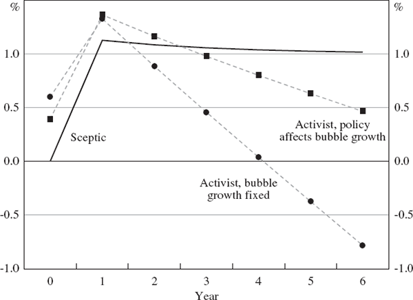
Notes: The probability of the bubble bursting is pt = 0.4. The sceptic implements policy in each year. Real interest rates are deviations from neutral.
For every year apart from year 0, being able to reduce the bubble's growth induces the activist policy-maker to recommend tighter policy than she otherwise would.
The differences in the policy recommendations induced by this expectation are, however, less pronounced than the differences that arise when an activist policy-maker assesses the probability that the bubble will burst each year at pt = 0.2 rather than pt = 0.4, as can be seen by comparing Figures 1 and 5.
3.2.4 Bubbles that take two or more years to collapse
Another extension to the basic model involves assuming that, when the bubble collapses, it does so evenly over two or more years, rather than suddenly in one. In the examples we have examined until now, the activist must always confront the problem that, owing to the lag structure of the Ball model, policy can only respond to a collapsing bubble after the collapse is complete. This problem is reduced by assuming that the collapse occurs over two or more years rather than one.
Figure 6 shows results for the sceptic and two activists (one who assumes gradual, even, two-year collapse; the other, sudden), assuming that pt = p* = 0.4 (except p14 = 1) and that γt = 1. The activist who assumes that the bubble will collapse only gradually recommends tighter policy than the one who assumes that it will be sudden, because of their different assessments of the bubble's expected effect on next year's output.
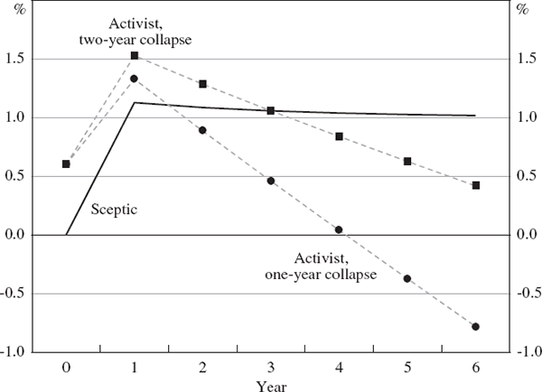
Notes: The probability of the bubble bursting is pt = 0.4. The sceptic implements policy in each year. Real interest rates are deviations from neutral.
Nevertheless, the overall pattern of policy recommendations remains similar to earlier cases. As the size of the bubble grows, the ‘gradually-bursting’ activist eventually recommends looser policy than the sceptic does, for reasons that are by now familiar.
In cases in which the bubble is expected to collapse evenly over three or more years, the activist would recommend tighter policy than the sceptic for longer, while the bubble is growing, a result that follows from a straightforward extension to Equation (8).
3.2.5 A rational bubble
In the baseline results presented at the beginning of the section, we assumed that the asset-price bubble grew at a uniform rate, γt = 1, and that the probability of the bubble's collapse was constant through time. This seems to us a simple and intuitively appealing baseline case.
In this case, however, there is no arbitrage condition ruling out unexploited profit opportunities in the assets whose price rises constitute the bubble. Our baseline case is therefore not a ‘rational’ bubble. We do not see this as a shortcoming – to our minds, there is much evidence that the asset-price bubbles we see in modern industrial economies are not rational in this sense (see, for example, Shiller (2000)). Nevertheless, it is of interest to derive results for the case of a rational bubble.
Such a bubble arises from the actions of a rational investor who buys the relevant assets up to the point at which expected profits are driven to zero.[13] If the probability of collapse is constant, p*, and the capital gain to the investor in year t + 1 if the bubble collapses is −αt, then a rational risk-neutral investor will be indifferent to holding the asset when the expected growth of the bubble, if it survives, is Δαt+1 = αtp*/(l − p*). This is a geometrically growing bubble, rather than the constant-growth bubble that constituted our baseline case.[14]
The arbitrage condition that defines this rational bubble implies that the bubble's expected
growth over the next year,  , is zero. In this case, however, the
activist and the sceptic are making identical assumptions about the bubble's expected effect
on next year's output. It follows that the activist will always recommend the same policy
interest rate as the sceptic for a rational bubble, provided she believes that the stochastic
properties of the bubble are not affected by the actions of policy-makers, so that certainty
equivalence holds.[15]
Footnotes
For completeness, Appendix A shows optimal interest rate recommendations both before and after the bursting of the bubble. [5]
The model set-up is more complex than the standard set-up in which certainty equivalence
applies. This is because, once the bubble bursts, there are no further asset-bubble
shocks and hence, ex ante, the distribution of shocks is not
independent through time. It is, therefore, not straightforward to demonstrate certainty
equivalence. Nevertheless, Equation (8) in the text does follow and can be generalised
to allow for alternative parameter values, time-varying bubble growth and/or
probabilities of bubble collapse, provided that the evolution of the bubble remains
independent of the actions of the policy-makers. The generalised equation is  which, in particular, implies that (
 –
–  )
does not depend on α, λ or μ. A proof of this
equation is provided in Appendix C.
[6]
Assuming pt = 0.2 implies an average remaining life for the bubble of five years, while pt = 0.4 implies an average remaining life of two and a half years. [7]
Most of the extensions we examine in this section imply that certainty equivalence no longer applies to the model (the exceptions are the bubble that collapses over two or more years and the rational bubble), in which case the results must be derived by numerical optimisation. To simplify the numerical problems, we assume that if the bubble survives until year 14 (which is a very unlikely event for all the parameter values we consider) then it bursts with certainty in that year. For earlier years, this assumption is only relevant for the policy choices of the activist policy-maker. [8]
We choose the functional form in Equation (9) so that, for the benchmark policy settings chosen by the sceptic, pt = p* for all t. The results generated using an alternative functional form, pt = p* + δrt−1, are qualitatively very similar to those shown. [9]
It seems implausible that moderate rises in the real interest rate would burst the bubble with certainty; yet that is an implication of the linear form, Equation (9). Simulations of the linear model with δ > 0.1 do indeed generate this outcome (results not shown). It is for this reason that we use the non-linear form for simulations with δ > 0.1. As argued by Stockton (2003), one could also imagine that the relationship between the bubble's probability of collapse and the policy interest rate might be non-monotonic, with small interest rate rises lowering the subsequent probability of collapse. This would undoubtedly further complicate the optimal policy recommendations of an activist. [10]
If the bubble survives, it would again be necessary to set policy 1 percentage point higher than the sceptic to ensure that the bubble did not grow in the subsequent year. Given the effects of continually tight policy on the rest of the economy, it is perhaps not surprising that being able to raise the probability that the bubble will burst has more influence on optimal policy than simply being able to reduce its growth each year by setting tighter policy in each previous year. [11]
The results assuming no interest-rate sensitivity are equivalent to the baseline results shown in Figure 1 for the activist assuming pt = 0.4. [12]
We assume that the assets yield an annual return equal to the real interest rate, so that the expected profit relative to holding 1-year government bonds is determined by the expected capital gain on the assets. [13]
Note that, if the probability of collapse is not constant, a rational bubble need not grow at a constant geometrical rate. [14]
This result relies on a number of implicit, simplifying assumptions about the economy. In particular, it relies on the assumptions that the effect on the output gap of changes in asset prices is proportional to the size of those changes, and that rational investors and the activist policy-maker agree on the exact stochastic details of the bubble. Relaxing either of these assumptions could generate different policy recommendations by the activist. For example, for a geometrically growing bubble, it could account for an activist policy-maker assessing the bubble's growth rate to be faster (slower) than ‘rational’ – say, Δαt+1 = χαtp*/(1 − p*), with χ > 1 (χ < 1) – in which case the activist's policy recommendations would always be tighter (looser) than the sceptic's, for as long as the bubble survived. [15]


