RDP 2005-07: The Australian Business Cycle: A Coincident Indicator Approach 6. Applications of the Coincident Indices
October 2005
- Download the Paper 1.72MB
6.1 The Decline in Volatility
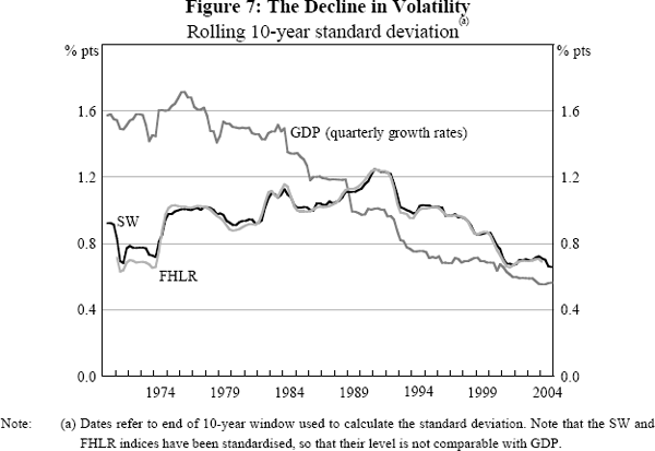
Simon (2001) documents the decline in the volatility of quarterly GDP growth over the past 45 years that was evident in Figure 1. Figure 7, which plots the rolling standard deviation of quarterly GDP growth calculated over 10-year windows, also demonstrates this decline in volatility. Interestingly, and in contrast, the 10-year rolling standard deviations of the SW and FHLR indices display no marked trend in volatility over the full sample.[12]
To better understand this divergence in trends in volatility, we focus on the SW index and the series used in its compilation, since it is simply a weighted average of the data in each quarter. The variance of the coincident index, which for the SW index is simply the first factor, can be decomposed into the variances and covariances of the series used in its construction. First, note that a factor can be expressed as a weighted average of the data, as given by Equation (2),
where ci is the weight on the ith series, xi. The variance of the factor can then be decomposed as the weighted sum of the variances of the component series and their covariances, as given by Equation (3):
Given that the volatility of quarterly GDP has declined substantially, we decompose the volatility of the SW factor separately into the variances and covariances of the 6 national accounts series and the 19 other series. We calculate the variances in two sub-samples, before and after 1980, which is close to the middle of the full sample period and avoids splitting during a recession (Table 5).[13]
| Variance terms | Covariance terms | Variance of SW index |
Variance of GDP |
|||||
|---|---|---|---|---|---|---|---|---|
| National accounts | Other | National accounts | Other | National accounts/other | ||||
| 1960–1979 | 0.07 | 0.11 | 0.14 | 0.36 | 0.34 | 1.03 | 2.45 | |
| 1980–2004 | 0.04 | 0.11 | 0.08 | 0.36 | 0.33 | 0.92 | 0.63 | |
| Note: The scaling ensures the SW factor has unit variance over the full sample. | ||||||||
Confirming the picture suggested by Figure 7, the variance of quarterly GDP growth in the latter sample is around a quarter of its variance in the first sample (the last column of Table 5). In contrast, the variance of the SW index is little changed (column six). The first five columns in Table 5 give the weighted variances and covariances that sum to the variance of the SW index. The weighted sums of the variances and covariances of the national accounts series used in the SW index declines by about one-half (this is less than the decline in GDP volatility because the two capital formation series included in our index experienced an increase in volatility).[14] In contrast, the weighted sums of the variances and covariances of the 19 other series used in the SW index are virtually unchanged, as are the covariances between the national accounts and other series. In total, the SW index has only a minor decline in volatility because the other economic series (which cumulatively have a greater weight in the SW index) did not experience the same decline in volatility as the national accounts aggregates. To the extent that the coincident index provides a good indicator of the business cycle by abstracting from idiosyncratic noise in individual series, this suggests that the decline in the volatility of the common component of economic activity has not been as marked as indicated by quarterly estimates of GDP. If the analysis of volatility is performed using annual growth rates, the decline in the standard deviation of GDP is less dramatic but is still apparent, at least over the latter half of the sample.
Again, the SW index shows no decline in volatility and the findings from decomposing the volatility of quarterly movements in the SW index carry over to the decomposition using annual changes.
One possible explanation for the divergent trends in volatility is that some of the volatility in GDP in the earlier part of the sample reflects measurement error and that the SW index is able to abstract from such idiosyncratic noise. As GDP has become better measured over time, the volatility of measured GDP has declined.[15] Harding (2002) provides further discussion on the decline in the volatility of GDP in Australia, suggesting that it largely reflects reduced measurement errors, and in particular less residual seasonality.[16] It may be that other series, such as employment or dwelling approvals, have not had this reduction in measurement error because they have always been easier to measure than GDP. A second explanation is that it may be that the parts of the economy that have experienced a decline in volatility are under-represented in the panel. This would seem less likely as one of the main criteria for selecting the panel of data series is that it should provide a broad representation of the economy. In addition, the magnitude of the decline in sectoral volatilities (or shifts in sectoral shares) that would be required to explain the decline in GDP volatility seems somewhat implausible.
Given the volatility of some economic series has changed it may be that the importance of various series in the construction of the coincident indices has also changed. To examine this, we estimate the SW index over the two sub-samples, 1960–1979 and 1980–2004, using the panel of data that is available over the full 1960–2004 sample.[17] As Figure 8 shows, the coincident indices estimated over the two sub-samples are virtually identical to the index constructed over the full sample. The only visible difference is that the SW index, estimated over the full sample, has a slightly positive (negative) mean over 1960–1979 (1980–2004) while the two sub-sample indices have zero mean by construction; this reflects the higher average economic growth in the 1960s.
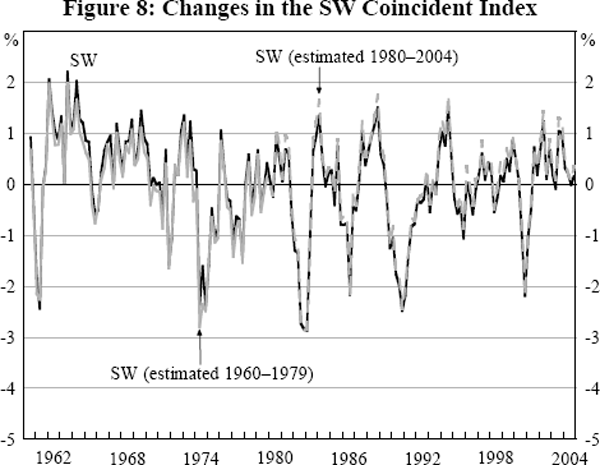
Not surprisingly, given the insignificant change in the coincident index, the weights used to estimate the factors are little changed when the shorter sub-samples are used. Indeed, the panel R-squared for the first factor increases only marginally from 0.231 to 0.257, demonstrating that, for the panel as a whole, idiosyncratic shocks have declined only marginally.[18]
6.2 Dating the Business Cycle
In this section, we use the coincident indices to date classical cycles, that is cycles involving a decline in activity rather than just a slowing in growth rates. To identify periods of recession, we use the Bry and Boschan (1971) algorithm. This is an NBER-style rule that identifies the peaks and troughs in the level of a series and so dates expansions and contractions in an objective manner. Appendix B provides further details on the procedure, including the construction of a levels series from the SW index.
Table 6 reports the recessions identified by GDP and the quarterly SW and FHLR indices.[19] While six recessions are located by GDP, only three recessions are identified by the two coincident indices. The three recessions that GDP identifies, but the indices do not, occur in the mid 1960s, and early and late 1970s. As discussed in Section 6.1 the volatility of quarterly GDP growth has declined, while the coincident indices that are based on many series (and statistical weights) have not seen such a reduction in volatility. The greater number of recessions that are identified by GDP appears to be the result of its higher volatility early in the sample. Assuming no change in mean growth rates, higher volatility of measured GDP growth would tend to increase the likelihood of recording (possibly spurious) declines in the level of GDP, and so of recessions being identified in the data.[20] Alternatively, we could date the business cycle using non-farm GDP to abstract from the possibility that the volatile farm sector could result in declines in aggregate GDP even when there was no decline in the broader non-farm economy. Unlike GDP, non-farm GDP does not locate recessions in 1965–1966 and 1971–1972, but it does identify the other recessions found in GDP, and an additional recession in the mid 1980s (1985:Q4–1986:Q2). So, abstracting from farm output does reduce the number of recessions identified, but still results in more recessions than the three identified by the coincident indices.
| Quarterly | Monthly | |||||||
|---|---|---|---|---|---|---|---|---|
| 1960–2004 | 1960–2004 | 1980–2004 | ||||||
| GDP | SW | FHLR | Melbourne Institute | SW | FHLR | |||
| Peak | 1965:Q2 | |||||||
| Trough | 1966:Q1 | |||||||
| Peak | 1971:Q3 | |||||||
| Trough | 1972:Q1 | |||||||
| Peak | 1975:Q2 | 1974:Q1 | 1974:Q1 | 1974:M7 | ||||
| Trough | 1975:Q4 | 1975:Q1 | 1975:Q1 | 1975:M10 | ||||
| Peak | 1977:Q2 | 1976:M8 | ||||||
| Trough | 1977:Q4 | 1977:M10 | ||||||
| Peak | 1981:Q3 | 1981:Q4 | 1982:Q1 | 1981:M9 | 1982:M5 | 1982:M2 | ||
| Trough | 1983:Q1 | 1983:Q1 | 1983:Q1 | 1983:M5 | 1983:M1 | 1983:M3 | ||
| Peak | 1990:Q2 | 1990:Q1 | 1990:Q1 | 1989:M12 | 1990:M7 | 1990:M5 | ||
| Trough | 1991:Q3 | 1991:Q2 | 1991:Q1 | 1992:M12 | 1992:M5 | 1991:M8 | ||
| Note: The Melbourne Institute business cycle dates are an update of those in Boehm and Moore (1984). | ||||||||
Overall, we conclude that using a broad panel of series provides less evidence that the GDP downturns in the mid 1960s and early and late 1970s were recessions, but that three recessions are unambiguously identified, in 1974–1975, 1982–1983 and 1990–1991. These three recessions occurred at times when most industrialised countries experienced recessions.[21]
The recession dates produced by the Melbourne Institute (which follow on from the work by Ernst Boehm and Geoffrey Moore) are also given in Table 6. These dates are based on several monthly and quarterly series, but not as many as the SW and FHLR indices. Like these indices, the Melbourne Institute does not date 1965 and 1971 as being recessions. However, they do consider 1976 to have been a recession. This implies that there was an expansion in 1975–1976 that lasted just 10 months.
The monthly SW and FHLR indices (which cover the period 1980–2004) also identify the early 1980s and early 1990s as periods of recession (columns five and six of Table 6). The two indices imply similar timing for the early-1980s recession, but the SW index dates the end of the early-1990s recession nine months later than the FHLR index. This highlights the sensitivity of these monthly indices to the number of factors used to form the index. The SW index which only uses one factor picks up a different cycle to the common component from two factors – the two-factor SW index (q*=2) identifies similar turning points to the FHLR index.
The length of the three main recessions identified in the quarterly data differs only modestly according to whether the dating uses GDP, SW or FHLR. FHLR indicates that all three recessions were four quarters long, while for GDP they range between three and six quarters. In contrast, because GDP and the two indices identify different numbers of recessions, the lengths of the expansions identified differ greatly (Figure 9). Since the use of GDP suggests there have been more recessions, it identifies expansions as being shorter on average, with one lasting only six quarters. This follows from the extra recessions identified by GDP in the 1960s and 1970s, which appear to be the result of the higher level of noise in GDP. The smoother FHLR and SW indices identify a long expansion at the beginning of the sample, two expansions of about seven years each in the middle, and then another ongoing long expansion.
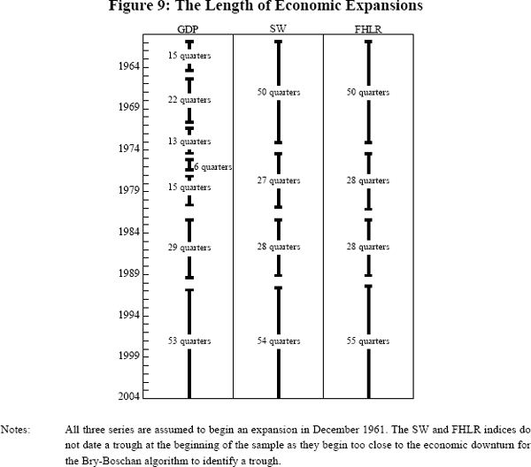
Figure 10 plots GDP along with three representative series – GNE (to capture domestic demand), employment, and the ACCI-Westpac survey of actual output (to capture production) – and highlights the three recessions identified by the SW and FHLR coincident indices. The economic downturn in the three recessions was widespread. In all three recessions, not only did GDP contract, but domestic demand fell, the net balance of actual output from the ACCI-Westpac survey was strongly negative, employment experienced sustained falls, and the unemployment rate increased by over 3 percentage points. The fall in GDP was less severe in the 1974 recession. Indeed, as shown in Appendix C, various vintages of GDP have not identified this as being a recession. However, both coincident indices strongly identify this episode as being a recession. To reconcile these facts we note that while private demand and production (and, therefore, many of the series in our data panel) experienced a significant downturn, there was a substantial boost in public expenditure, offsetting much of the decline in the other components of GDP. But given the widespread decline in economic activity it seems reasonable to characterise this episode as a recession.
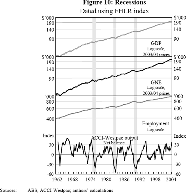
The end of all three recessions marks the end of the sharp decline of demand, and coincides with the turnaround in the ACCI-Westpac survey. While the recovery in employment also dates from the end of the 1970s and 1980s recessions, employment was weak for a sustained period after the 1990s recession. These disparate trends in different variables around the 1991 recession appear to explain the sensitivity of the monthly SW index to the number of factors used in its construction.
In contrast, in the other three recessions identified by GDP, the downturn was not as uniform across different economic variables.[22] In 1965, employment continued to grow, GNE fell only in one quarter, while the ACCI-Westpac survey continued to record a positive net balance of respondents. In 1971, GNE did contract, and the ACCI-Westpac actual output net balance fell, though not by as much as in the three recessions. However, employment fell in only one quarter and there was still reasonable strength in housing and construction. So there is some evidence of a contraction in economic activity, but it was not widespread. In 1977, once again, GNE fell while employment fell in only one of the quarters. But the ACCI-Westpac survey was only slightly negative and investment and exports showed no sign of a downturn.
The constructed indices are less noisy measures of the business cycle than GDP, especially in the early part of the sample, suggesting that there are advantages from using a large range of series and a statistically based set of weights. Notwithstanding the fact that GDP has become less noisy over time, we conjecture that these advantages may also carry over to real-time analysis (though without real-time data for the series used to construct the indices we cannot test this conjecture). Some of the series used in the construction of the indices are not revised, and those series that are revised come from a range of different surveys or collection methods, so that revisions to particular series may be largely independent (and therefore mostly ‘wash out’). In addition, as shown in Section 6.1, the weights in the indices are quite stable between the first and second halves of the sample. In contrast, as Appendix C shows, the identification and timing of recessions can change substantially with revisions to GDP, although it must be noted that the periods of most substantial revisions pre-date methodological improvements in the construction of GDP.
6.3 Changes in International Correlation of Business Cycles
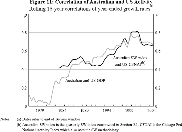
Another aspect of the changing nature of the business cycle is the extent to which correlations of cycles across countries may have changed, a topic which is addressed in Andrews and Kohler (2005), in a study using correlations of GDP. Our indices allow another perspective on this question. If the extent of measurement error in GDP changes over time, then this may alter the measured correlation of countries' business cycles. Comparing coincident indices across countries can provide a check on the extent to which measurement error might affect the measurement of synchronisation. Accordingly, Figure 11 shows the rolling correlation of annual rates of change in US and Australian GDP, and the correlation of the annual change in the Australian SW index constructed in Section 5.1 and the annual change in the Chicago Fed's US CFNAI (which is also constructed using the SW methodology).[23] These two rolling correlations demonstrate that the increase in the correlation of the Australian and US economic activity over the 1970–2000 period is robust to alternative measurement, suggesting that measurement issues are not a significant element in the changing correlation of the Australian and US business cycles.
6.4 The Relationships of the Indices with Other Economic Variables
We conclude the analytical part of this paper by considering how closely the quarterly indices estimated in Section 5 are correlated with a range of other more standard measures of the Australian business cycle, to get a better sense of exactly what our indices may be measuring. First, we compare the persistence (or first order autocorrelations) of our indices with the persistence of the quarterly change in GDP and some other standard variables. In principle, the concept of the business cycle is one of a relatively persistent process, so we would expect that a good measure of the cycle should have a relatively high degree of persistence.
Both the SW and FHLR indices have a high degree of persistence over the full sample, even at a quarterly frequency, with autocorrelations of 0.67 and 0.88, respectively (Table 7). By contrast, the standard national accounts aggregates display little persistence, with quarterly growth in GDP and non-farm GDP displaying negative autocorrelation, at least in the early part of the sample. In the later part of the sample, quarterly changes in the national accounts aggregates have become more persistent, but they are still much less persistent than the two coincident indicators. For year-ended growth rates the difference in persistence remains, though it is less marked (not shown). In short, the indices appear to be a better measure of the persistent economic cycle than is GDP, or other national accounts aggregates – certainly historically and, to a lesser extent, more recently.
| GDP | Non-farm GDP | DFD(a) | SW | FHLR | |
|---|---|---|---|---|---|
| Autocorrelations | |||||
| 1960–2004 | −0.07 | −0.07 | 0.04 | 0.67 | 0.88 |
| 1960–1979 | −0.22 | −0.19 | −0.08 | 0.58 | 0.86 |
| 1980–2004 | 0.34 | 0.10 | 0.17 | 0.73 | 0.88 |
| Correlations | |||||
| GDP | 1 | 0.77 | 0.50 | 0.62 | 0.45 |
| Non-farm GDP | 1 | 0.60 | 0.64 | 0.48 | |
| DFD | 1 | 0.69 | 0.55 | ||
| SW | 1 | 0.91 | |||
| FHLR | 1 | ||||
|
Notes: Correlations are for the full sample 1960–2004. (a) DFD is domestic final demand. |
|||||
Second, we consider how closely our indices are correlated with some national accounts measures, to get a slightly better sense of exactly what aspect of the business cycle they may be capturing. Although the panel of variables used to estimate the coincident indices was constructed to be as representative of the economy as possible, it does not have the coverage of measures of income, production or expenditure components which together are used to construct GDP. We expect that the common cycle estimated by our indices will be closely related to GDP, given that many of the series used to construct the indices are related to GDP or its components. Even so, it is possible that they bear a closer resemblance to other national accounts aggregates. The bottom panel of Table 7 shows that this is indeed the case. The two quarterly coincident indices have a marginally higher correlation with non-farm GDP than GDP, and a higher correlation still with domestic final demand. This ordering of correlations also holds for annual growth rates (not shown). In the latter part of the sample the correlation of the national accounts aggregates with the FHLR index in particular has increased, but the relative rankings of correlations have not changed. Even though the coincident indices are closely related to GDP, at times differences are apparent. As mentioned in Section 5.1, the coincident indices have been notably stronger than GDP growth over the past few years.
The higher correlation with non-farm GDP is perhaps not surprising, given that the contribution of the farm sector to GDP is highly volatile and often uncorrelated with other sectoral developments. This result would lend support to the idea that developments in non-farm GDP sometimes give a better sense of general trends in the economy than does aggregate GDP, which is implicit in the frequent use of non-farm GDP in much analysis by official sector and private sector economists. The finding of a higher correlation with domestic final demand is perhaps more surprising. One explanation could be that production variables are under-represented in our panel. Alternatively, it may be that short-term shocks to production that show up in GDP are not in the common cycle because they have a limited effect on a range of expenditure decisions by households and firms which depend more on expectations about permanent incomes.
Footnotes
This feature is not repeated with US data. The rolling standard deviations of the Chicago Fed's CFNAI, which uses the SW methodology, are very similar to those of US GDP. [12]
The results are broadly unchanged if we end the second sample in 1999 to abstract from the impact of the GST on variances and covariances. [13]
In the case of dwelling investment, this is the result of large movements in the year the GST was introduced, but for total capital formation, the increase in volatility occurred more broadly through the sample. [14]
There have been a number of improvements in the construction of the national accounts. These include: the improved methodology for constructing price estimates after the high inflation of the 1970s highlighted problems with the earlier series; the introduction of explicit balance of payments timing adjustments for major commodities from the late 1970s; dating trade flows according to the shipment date rather than the date of recording within the Customs system (backcast to the early 1980s); the development of an import price index (IPI) to replace the RBA's IPI that was based on export price indices of major trading partners (from the early 1980s); improvements in the profits survey in the early 1980s; and the revamping of the government finance system in the mid 1980s. Many of these initiatives apply to the data from the 1980s onward, suggesting that they may be a factor in the decline in volatility observed around this time. We thank the ABS for bringing to our attention the nature of these changes. [15]
However, the ABS examined the issue of residual seasonality and introduced new seasonal factors to address this problem with the release of the June 2002 national accounts. [16]
We do not report sub-sample estimates using the FHLR methodology as the conclusions do not differ. [17]
This is true even if we consider more factors. For example, the panel R-squared for four factors only increases from 0.515 to 0.535. [18]
As discussed in Appendix B, the dates for the SW index are sensitive to the choice of a scaling parameter. This does not affect the dates for the FHLR index. [19]
For a recession to be identified there will have to be a decline in GDP in at least one quarter. The probability of a fall in GDP will be higher if the volatility of quarterly GDP growth is higher, so making the identification of a recession more likely. [20]
Out of 12 other OECD countries contained in the Economic Cycle Research Institute dating, 10, 11 and 12 experienced recessions within 18 months either side of the 1974–1975, 1982–1983 and 1990–1991 recessions in Australia. [21]
Further discussion of these earlier slowdowns, along with evidence on behaviour of other economic variables is provided in RBA (1997), pp 4–6. [22]
Note that Andrews and Kohler (2005) use a more advanced measure of the correlations based on band-pass filters rather than growth rates as used here. For the US-Australian correlation of GDP these techniques deliver qualitatively equivalent results. We use the correlation of growth rates as the coincident indices have already been filtered and so are not level variables. [23]

