RDP 2005-07: The Australian Business Cycle: A Coincident Indicator Approach 5. Results
October 2005
- Download the Paper 1.72MB
In Section 5.1 we present the coincident indices constructed with quarterly data for the period 1960–2004, and analyse their robustness to alternative specifications. In Section 5.2 we present the indices constructed with monthly data for the period 1980–2004, and consider their robustness.[4]
5.1 Quarterly Coincident Indices
The coincident indices constructed with the SW and FHLR methodologies – using the quarterly balanced panel from 1960 to 2004 – are shown in Figure 1. Recall that most series used to derive the factors are log differenced and so the index has a natural interpretation as a quarterly growth rate of the economy (scaled to have mean zero and standard deviation of one). The SW index is estimated with no lags so that each value is a function of only the contemporaneous data (and constant weights which are estimated using the full sample). However, if the common component is sufficiently persistent it may not matter too much if some series are slightly leading or lagging. Providing that the leads and lags are short compared to the length of the common cycle, these series will still help to provide an estimate of the common cycle, despite not being perfectly aligned.
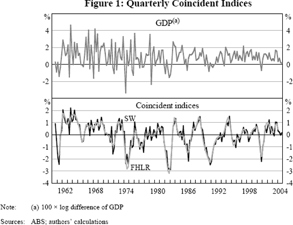
As discussed in Section 3, an information criterion can be used with the SW methodology to determine the number of factors required to explain the panel. The information criterion finds that there is only one factor, and so our SW index is simply the first factor, that is the first principal component. This first factor explains 23 per cent of the variation in the panel of 25 series. For the FHLR index, the explanatory power threshold selects two factors. These two factors explain 37 per cent of the total variance in the panel.
As can be seen in Figure 1, the two indices are very similar; indeed their correlation is 0.91. The most apparent difference is that the FHLR index is somewhat smoother because it removes high-frequency volatility by construction (as is discussed further below). Note also that the FHLR index is shorter by three quarters at both its beginning and end, because it requires leads and lags to estimate the spectral density matrix.
Both series are substantially smoother than quarterly changes in GDP (throughout we use 100 × log difference of GDP, to be consistent with the log differences used in the construction of the indices). It is not surprising that the FHLR index is less volatile than GDP as it is constructed as a two-sided filter, that is, using data either side of a given quarter to provide a smoother indicator, and is additionally smoothed by removing high-frequency movements. But the value of the SW index in a given quarter is constructed from only data in that quarter – it is not smoothed in any way other than the fact that it uses the cross-section of data. Further, the SW index uses only the first factor, while the FHLR index is an average of two factors.
There are clear economic cycles in the two constructed coincident indices, while it takes a more highly trained eye to discern a cycle in the quarterly changes in GDP. Both of our indices show three major downturns in economic activity over the 45-year period; in the mid 1970s, the early 1980s and the early 1990s. Smaller economic downturns show up clearly in the early and late 1970s, the mid 1980s, and a spike down in 2000 associated with the introduction of the GST. The long boom of the 1960s is evident with both indices around one standard deviation above zero for much of the decade. The past ten years or so have also seen the indices being positive on average, indicating stronger-than-average economic conditions.
Annual growth rates are often used to get a smoother picture of GDP growth. However, Figure 2 shows that annual GDP growth is still much noisier than the annual change in the SW index (the four-quarter sum, scaled to have the same mean and variance as annual GDP growth). The FHLR index is not shown since the annual changes are almost identical to those of the SW index.
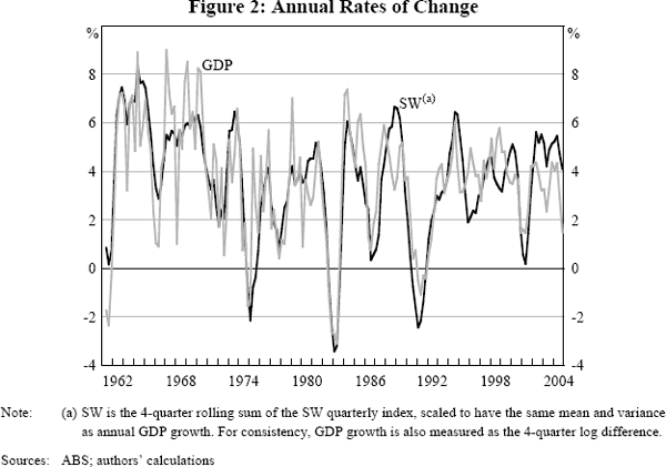
While the scaled growth in the SW index is typically around the same rate as GDP, differences do open up at times. Indeed, the SW index has been notably stronger than GDP growth over the past few years. This presumably reflects the relative importance of some series that have been very strong over this period (including employment and domestic demand).
5.1.1 Robustness of the quarterly indices
As discussed in Sections 2 and 3, the number of factors that are combined to form an index, and the composition of the panel used for estimation, will influence the behaviour of that coincident index. We examine the sensitivity of the SW and FHLR indices along these two dimensions.[5] Firstly, we construct both indices using alternative numbers of factors. Secondly, both indices are estimated using a much broader panel of 76 series that are available from 1980. We also examine the sensitivity to the breadth and composition of the panel by using even broader panels that are not balanced (that is they contain some missing observations) which can be used with the SW methodology. The non-balanced panels starting in 1960 and 1980 contain 68 and 111 series, respectively.
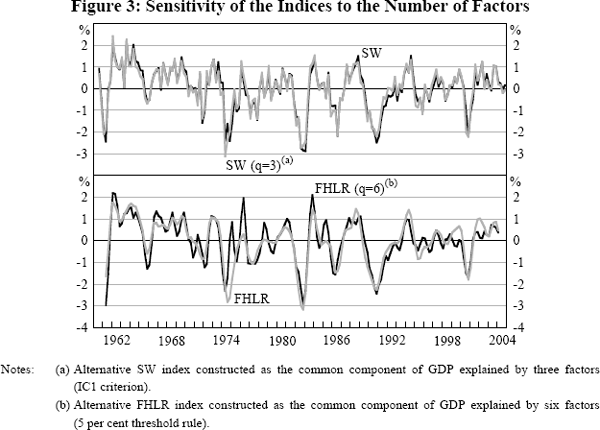
The information criterion for the SW index shown in Figure 1 selects one factor. However, an alternative information criterion proposed by Bai and Ng (2002), the IC1, selects three factors. As shown in the top panel of Figure 3, the coincident index constructed as the common component of GDP explained by the first three factors is very similar to, though slightly more noisy than, the one-factor SW index. The similarity implies that the extra two factors may be useful in explaining the panel of data, but do not contain much incremental explanatory power for GDP relative to the first factor. Adding more factors tends to make the index less persistent, that is, more noisy. The correlations of the alternative coincident indices, and their autocorrelation coefficients, are reported in Table 2.
| GDP | SW | FHLR | Alternative indices | |||||
|---|---|---|---|---|---|---|---|---|
| SW | FHLR | |||||||
| q=3(a) | NBP q=1(b) | q=1(c) | q=6(d) | |||||
| GDP | 1 | 0.62 | 0.45 | 0.64 | 0.52 | 0.44 | 0.53 | |
| SW | 1 | 0.91 | 0.97 | 0.95 | 0.92 | 0.81 | ||
| FHLR | 1 | 0.90 | 0.90 | 0.99 | 0.86 | |||
| SW (q=3) | 1 | 0.88 | 0.89 | 0.81 | ||||
| SW (NBP q=1) | 1 | 0.92 | 0.78 | |||||
| FHLR (q=1) | 1 | 0.84 | ||||||
| FHLR (q=6) | 1 | |||||||
| Autocorrelation | −0.07 | 0.67 | 0.88 | 0.64 | 0.80 | 0.88 | 0.77 | |
|
Notes: (a) SW common component using three factors (b) SW first factor from the non-balanced panel (c) FHLR first factor (d) FHLR common component using six factors |
||||||||
The second panel of Figure 3 plots the FHLR index against an alternative constructed using six factors, the number selected if the explanatory power threshold is set to 5 per cent rather than 10 per cent. Again, the series are very similar but, as with the SW indices, the alternative index constructed with more factors is less persistent. The result that the SW index gains little by using more than one factor also carries over to the FHLR index. The FHLR first factor has a correlation of 0.99 with the FHLR index that is the common component of two factors and is equally persistent (the autocorrelation of both is 0.88). We continue with the common component using two factors as our FHLR index, because it derives from the criterion used in the literature, but note that the results in the remainder of the paper are virtually identical if the FHLR first factor is used as the coincident index. In general, for other sample periods and panels of data, using more factors changes the common component little, but does tend to make it slightly more noisy (as seen by the smaller autocorrelation coefficients in Table 2). This raises questions about the benefits of adding additional factors in studies such as this one, in which we are interested in characterising the business cycle.
Using a broader, non-balanced, panel with 68 series for the period 1960–2004 also makes little difference to the estimated SW coincident index. The alternative SW index estimated with this broader panel has a correlation of 0.95 with the SW index (column 5 of Table 2).[6]
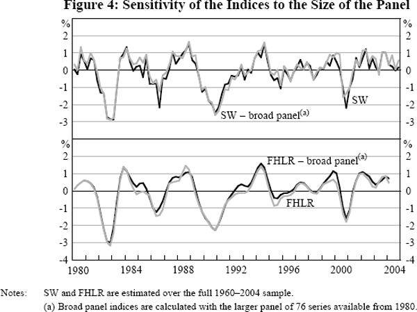
An alternative test of the impact the breadth of the panel has on the coincident indices comes from the use of the broader balanced panel of 76 series available over the period 1980–2004 to estimate the indices. Figure 4 plots the SW and FHLR indices against these alternative indices. These alternative indices differ from our two main indices along two dimensions; they use a panel containing over twice as many series, and they are estimated over a shorter period. Despite this, they are almost identical to our two main indices; the correlation of the two SW indices is 0.96 and the correlation of the two FHLR indices is 0.98, as reported in Table 3. Note that the difference between the two SW and two FHLR indices in Figure 4 is slightly exaggerated because the SW and FHLR indices estimated from 1960 have a small negative mean and standard deviation marginally less than one when plotted over the period 1980–2004. Broadening the panel further to estimate the SW index with the 111 series in the non-balanced 1980 panel similarly has little impact on the estimated index (column 5 of Table 3). This series has a correlation with the SW index of 0.95 and is only slightly smoother.
| GDP | SW(a) | FHLR(a) | Alternative indices (broad panel) | ||||
|---|---|---|---|---|---|---|---|
| SW | FHLR | ||||||
| q=1(b) | NBP q=1(c) | q=2(d) | |||||
| GDP | 1 | 0.68 | 0.62 | 0.68 | 0.66 | 0.64 | |
| SW | 1 | 0.94 | 0.96 | 0.95 | 0.93 | ||
| FHLR | 1 | 0.92 | 0.90 | 0.98 | |||
| SW (q=1) | 1 | 0.99 | 0.93 | ||||
| SW (NBP q=1) | 1 | 0.91 | |||||
| FHLR (q=2) | 1 | ||||||
| Autocorrelation | 0.36 | 0.73 | 0.88 | 0.77 | 0.80 | 0.88 | |
|
Notes: (a) Estimated over the period 1960–2004 (b) SW first factor using the broader 1980 balanced panel (76 series) (c) SW first factor using the broader 1980 non-balanced panel (111 series) (d) FHLR common component using two factors with the broader 1980 balanced panel (76 series) |
|||||||
5.2 Monthly Coincident Indices
For the period 1980–2004, we estimate SW and FHLR indices using a panel of 29 monthly series. The FHLR methodology requires the inclusion of GDP in the panel, and so to estimate the monthly FHLR index the panel of monthly data is augmented with GDP (with the growth rate in each month assumed to be one-third of the quarterly growth rate for each month in the quarter, as is standard in the FHLR methodology).[7] In contrast to the quarterly panel, the panel of monthly data has no national accounts series (household income, etc) and no measures of production. Rather it contains proportionately more overseas sector variables (trade, the exchange rate, etc) and private finance variables (credit, lending approvals, etc). Every effort is made to keep this panel as representative as possible, but given that some types of series are not produced at a monthly frequency they are obviously under-represented. The sensitivity to this constraint is considered in Section 5.2.1 with the construction of mixed-frequency indices that also include some of these quarterly series.
The quarterly SW index is estimated with no lags, as the series in the panel are taken to be mostly contemporaneously related at a quarterly frequency. This assumption is validated by the fact that FHLR places relatively small (and generally reasonably symmetrical) weights on leads and lags, and the close contemporaneous relationship of the FHLR index with the SW index. However, leads and lags are presumably more important in constructing a monthly index. To account for this we estimate the SW index using a stacked panel (with s=2 in Equation (1)). We interpret this model as having one lead and one lag, rather than two lags. This alignment of the index corresponds better with the path of the economic series and the FHLR index.
In a dynamic factor model, in which the data depend on leads and lags of the factors, the Bai and Ng (2002) information criteria will only provide an upper bound for the number of factors relevant for the model.[8] The IC2 information criterion selects two factors. However, the weight on the second factor in the regression of GDP on the two factors is very small and so we present the first factor as our monthly SW index (the correlation of the two-factor common component with the first factor is 0.99).[9] As for the quarterly index, the 5 per cent threshold criterion selects two factors for the monthly FHLR index. The SW and FHLR indices are substantially different, especially around the 1990s recession (Figure 5). These differences are almost entirely a function of the fact that the SW index uses only one factor while the FHLR index is a linear combination of two factors. The SW index displays the same timing and magnitude of movements as the FHLR first factor; while the SW and FHLR indices have a correlation of 0.60, the SW index and FHLR first factor have a correlation of 0.90.
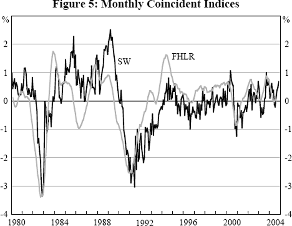
As already noted, the second SW factor has an insignificant weight when included in a regression of GDP on the factors. Similarly, the third factor has little correlation with GDP. In contrast, if both the first and fourth factors are used to explain GDP they have virtually identical weights. Indeed, the SW common component that uses just the first and fourth factors (which we report as q*=2) displays similar movements to the FHLR index (which also uses two factors). This alternative SW index that uses two factors has a correlation of 0.92 with the FHLR index. The second and third SW factors appear to be ‘nuisance’ factors which result from the use of a stacked panel.[10] While the business cycle could be well characterised by one factor for the quarterly panel of data, in the monthly case there are two factors that each represent different cycles, and so a common component of the two may better characterise the business cycle. The main difference between the SW and FHLR indices that use the same number of factors is that FHLR indices are smoother, largely because, by construction, they remove high-frequency volatility. This comes at the expense of the estimation procedure truncating the beginning and end of the sample. The FHLR index also incorporates information from four leads and four lags while the SW index has just one lead and one lag.
5.2.1 Robustness of the monthly indices
As discussed in the previous section, the monthly coincident indices are sensitive to whether one or two factors are used in their construction, unlike the quarterly indices for which the cycle changes little with the use of more factors (though the amount of noise in the index does change). However, the indices do seem to be fairly robust to the use of more than two factors in their construction. For example, Table 4 shows that the monthly FHLR index, which uses two factors, has a correlation of 0.92 with the alternative FHLR index that combines six factors (the number determined by the 5 per cent threshold) and the persistence is essentially unchanged.
| SW | FHLR | Alternative indices | Westpac/MI(f) | |||||||
|---|---|---|---|---|---|---|---|---|---|---|
| SW | FHLR | |||||||||
| q*=2(a) | NBP r=1(b) | MF r=5(c) | q=1(d) | q=6(e) | ||||||
| SW | 1 | 0.60 | 0.71 | 0.88 | 0.64 | 0.90 | 0.53 | 0.51 | ||
| FHLR | 1 | 0.92 | 0.83 | 0.93 | 0.84 | 0.92 | 0.61 | |||
| SW (BP q*=2) | 1 | 0.87 | 0.94 | 0.91 | 0.78 | 0.59 | ||||
| SW (NBP r=1) | 1 | 0.87 | 0.93 | 0.70 | 0.60 | |||||
| SW (MF r=5) | 1 | 0.81 | 0.78 | 0.62 | ||||||
| FHLR (q=1) | 1 | 0.77 | 0.59 | |||||||
| FHLR (q=6) | 1 | 0.57 | ||||||||
| Westpac/MI | 1 | |||||||||
| Autocorrelation | 0.89 | 0.98 | 0.89 | 0.93 | 0.92 | 0.99 | 0.97 | 0.23 | ||
|
Notes: (a) SW common component using two factors; the first and fourth factors (q*
is used to indicate that we selected the factors) (b) SW first factor from the non-balanced panel containing 45 series (the total number of factors is denoted by r in the stacked panel) (c) SW common component using five factors from the mixed-frequency panel that adds 19 quarterly series to the balanced panel (d) FHLR first factor (e) FHLR common component using six factors (f) Westpac-Melbourne Institute Coincident Index of Economic Activity |
||||||||||
At the monthly frequency, the correlations of the coincident indices using alternative specifications are lower than at the quarterly frequency. However, the monthly SW index is quite robust to using a broader panel; for example, the SW index has a correlation coefficient of 0.88 with an alternative index using the non-balanced panel with 45 series that also only uses the first factor. The SW index is also robust to estimation with a mixed-frequency panel of the 29 monthly series and 19 quarterly series. In this case, the common component of five factors (as selected by the information criterion) is very similar to the FHLR index (Figure 6) and to the two-factor SW index, with correlations of 0.93 and 0.94.[11] This suggests that the inability to include national accounts series in the monthly panel does not distort the shape of the business cycle captured by the indices.
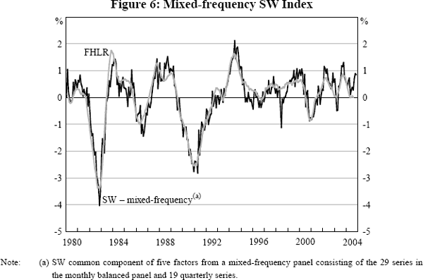
Table 4 also reports the correlations of SW and FHLR, and their various alternative specifications, with the Westpac-Melbourne Institute Coincident Index, a commonly cited monthly composite indicator in Australia. As discussed in Section 1, it is based on a simpler methodology and is noisier than the other coincident indices in Table 4, in part because it does not include leads or lags.
Footnotes
We would like to thank Robert Inklaar for providing Matlab code used to estimate FHLR, and Mark Watson, from whose website we obtained Gauss code used to estimate SW. [4]
We also examined the robustness of the indices to correction for outliers. Setting extreme values (say, those greater than four or ten times the interquartile range) to either missing values or maximum values generally has little effect on the estimated indices. The indices are also robust to using a panel of data in which large consecutive offsetting observations (for example a normalised growth rate of −5 per cent followed by +5 per cent), which possibly represent timing issues in the data, are smoothed. [5]
The information criterion selects three factors but we present the first factor for direct comparison with the SW index from the balanced panel. The common component using three factors has a higher correlation with GDP but is much more noisy, and is substantially less persistent than the first factor. [6]
As Caton (2005) notes, this series of constant growth in each month of the quarter will effectively lag the true underlying monthly growth in GDP by one month, an issue we had considered. We use this timing assumption as it has been used in the existing literature, and shifting the imputed monthly GDP growth forward by one month makes an indiscernible difference to the calculated index. [7]
In the SW setting this can be seen because the estimation technique does not recognise that ft and ft−1 are the same factors. Therefore, the information criteria will provide a guide to r rather than q. [8]
To determine the weights to combine the factors we regress GDP on the monthly factors. GDP is assumed to grow at one-third of the quarterly rate in each month of the quarter. This assumption is consistent with the assumption made about GDP growth in construction of the monthly FHLR index. [9]
The second and third factors have small weights when included in a regression of GDP on the first four factors. They are very noisy, with autocorrelation coefficients of −0.63 and −0.55. This is seemingly the result of using a stacked panel. We also find negatively autocorrelated factors, though weaker than for Australia, when stacking the panel used to construct the CFNAI. We thank Mark Watson and Jim Stock for discussing this point with us, and Watson for the following intuitive example. Suppose the data panel is explained by only one factor, which is positively autocorrelated, ft=ρ ft−1 + ηt. Then the stacked panel, which augments the data matrix with one lag, will be spanned by two factors. Since they must be orthogonal, if one factor is ft + ft−1 the other could be ft − ft−1. In this example, the second factor from the stacked panel will be negatively autocorrelated even though the true factor is not. [10]
The mixed-frequency SW index does not use interpolated quarterly data, unlike GDP used in the FHLR index. Rather, monthly values are calculated as functions of the factors, subject to the constraint that they ‘add up’ to the quarterly values. [11]