RDP 2006-02: Term Structure Rules for Monetary Policy 3. Equilibrium Determinacy

Under appropriate identifications, the model can be written in matrix form as

where: is a (m × 1) vector of pre-determined variables at t; p is a(n × 1) vector of non-pre-determined variables at t; and v_t is a (k × 1) vector of exogenous variables.^[11]

Let be the number of eigenvalues of K outside the unit circle. There are three cases to consider. If then there is a unique equilibrium solution. If then an equilibrium solution does not exist, and if then there is an infinite number of equilibrium solutions.^[12]

As the reader might appreciate, the study of uniqueness becomes analytically intractable, especially as we move towards larger maturities. For this reason, I resort to a numerical study of the problem. Nevertheless, as shown below, interesting numerical patterns emerge from this study.

3.1 Type-1 Rules: Reacting to Long-term Interest Rates

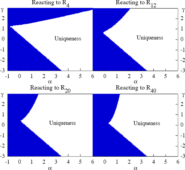
In this sub-section I study the conditions that support a unique REE for the class of type-1 rules given by R_1,t = τR_1,t−1 + απ_t + δx_t + γR_i,t. Figure 1 shows the regions of uniqueness for given values of τ and δ in the space of α and γ.^[13] A number of interesting features of this type of policy rule are worth highlighting.

Notice that the critical contour, for which the crucial eigenvalue of the K matrix is 1, has a downward- and an upward-sloping part in each case. The downward-sloping portion of the contour reveals that there is a trade-off, in terms of assuring a unique equilibrium, between the reaction to current inflation, α, and the reaction to the long-term nominal interest rate, γ.

Further numerical exploration shows that in the downward-sloping part of the contour, a condition of the form (τ + α + γ > 1) is necessary for determinacy, regardless of the maturity length in question. Note that the Taylor principle (α + τ > 1), that the short-term rate must rise sufficiently in the long run in response to movements in inflation so as to increase real rates, no longer holds in this case. The upward-sloping section of the contour shows that for a given α, as γ becomes ‘too large’, the policy rule is unable to produce a unique outcome. The intuition behind this result is the following. For simplicity, take the two-period interest rate and use Equations (1) and (2) to write

The above expression shows that by reacting to the two-period interest rate, the monetary authority is implicitly reacting to the average expected path of inflation in the following two periods. This explains why the Taylor principle is modified to a more general condition of the form (α + τ + γ > 1) in the downward-sloping part of the contour. In this sense there is a trade-off for assuring a unique equilibrium between the reaction to the long-term rate and current inflation.

To gain intuition about the upward-sloping portion of the contour, recall that, according to the expectations hypothesis, we may alternatively express R_2,t as

The problem is that a ‘too large’ value of γ allows self-fulfilling expectations to take place. To see why, observe that expectations that interest rates will be high become self-fulfilling, because the expectations of high short-term rates in the future causes long-term rates to rise, leading the monetary authority to raise short-term rates. Thus, in this case the monetary authority validates the initial expectation that short-term rates will be high. The upward-sloping part of the contour shows that there is a complementarity between α and γ. In this region, a higher value of γ requires a stronger response of the short-term rate to inflation in order to avoid the possibility of self-fulfilling expectations. It is in this respect that the Taylor principle breaks down for type-1 rules.

Further numerical exploration shows that in the upward-sloping part of the contour, higher values of τ and δ permit, for a given value of α, a higher value of γ. Notice that the Fisher decomposition implies, without loss of generality, that reacting positively to R₂ is equivalent to an implicit negative reaction to the current output gap. To see this, consider Equation (5), the type-1 policy rule with i equal to 2, and rewrite it with the help of the Fisher decomposition as

For this reason, higher values of δ allow for higher values of γ without implying a negative reaction to the current output gap.^[14]

Figure 1 reveals that as we move towards policy rules that involve larger maturity rates, the upward-sloping region of the critical contour increases its slope. So, for a given value of α it is possible to ensure unique solutions with even higher values of γ as the maturity lengthens. The fact that the interest rates in the policy rule are further apart in terms of maturity explains this result. When monetary policy reacts to very long-term rates, expectations can become self-fulfilling if the reaction of the short-term rate to this movement is sufficiently strong so as to feed through the term structure with enough strength to move the very long-term rate in a self-validating manner. So, as a stylised numerical observation, if the condition τ + α + γ > 1 is satisfied (for given values of the other parameters) the larger the maturity of the long-term rate in a type-1 rule, the larger the value of γ that supports a unique solution of the system.

Up to this point I have shown that there are large and empirically plausible regions of the parameter space for which type-1 rules yield a unique REE. This is important because rules that support multiple solutions are problematic. The mere fact that such a rule may be consistent with a potentially desirable equilibrium is of little importance if it is also equally consistent with other, much less desirable equilibria. A rule that implies indeterminacy is consistent with a large set of equilibria, including ones in which the fluctuations of endogenous variables are arbitrarily large relative to the size of fluctuations in the exogenous shocks.^[15] In general, variables for which there may be arbitrarily large fluctuations due to self-fulfilling expectations include those that enter the loss function of the monetary authority. Hence, at least some of the equilibria consistent with the rule are likely to be less desirable, in terms of the loss function, than the unique equilibrium associated with a rule that guarantees a unique solution.

For these reasons, the normative analysis restricts its attention to rules that imply a unique equilibrium. The question of the benefits of type-1 rules that yield a unique solution is taken up in Section 4.

3.2 Type-2 Rules: Long-term Interest Rate Rules

Here I study the conditions under which a unique REE exists for the class of type-2 rules given by R_i,t = τR_i,t−1 + απ_t + δx_t. In this case, a longer-term interest rate enters in the left-hand side of the reaction function used by the monetary authority. Recall that this does not imply that the monetary authority needs to change its operating procedures in any respect. The central bank can still use the short-term rate as its operating instrument to achieve the same equilibrium allocation. Rather, this is merely a more straightforward way to consider a rule which, when expressed in terms of the response of the short rate, can be quite complex.

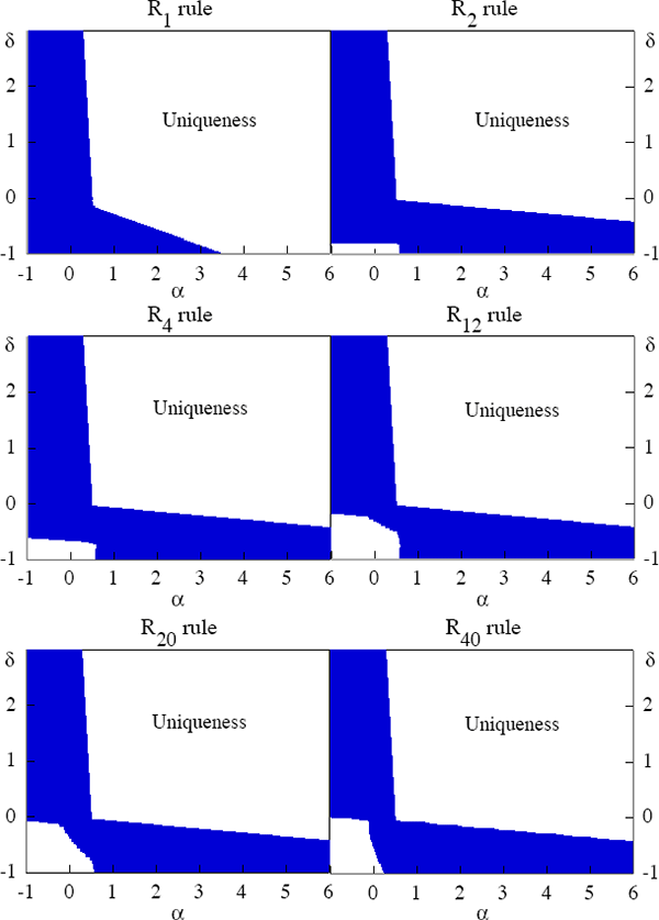
Figure 2 shows the regions in the space of α and δ in which a unique REE exists for τ = 1/2. As can be observed, significantly large regions of the parameter space exist that produce a unique REE.^[16] Notice that the regions of determinacy in the positive quadrants remain unchanged whatever the term of the interest rate chosen for the rule. Interestingly, Figure 2 also shows that, in the positive quadrants, the Taylor principle holds for the selected value of τ. Notice that α + τ > 1 is required for determinacy in these cases. In other words, for all rules and τ = 1/2;, determinacy of the REE requires α > 1/2. Although the numerical exercise so far suggests that the Taylor principle generalises to longer maturities, this is true only in some regions of the policy-parameter space.

Further exploration in the space of α and τ shows that the Taylor principle eventually breaks down for longer-term interest rates rules by displaying an upward-sloping section of the critical contour. This complementarity between α and τ shows up for sufficiently positive values of δ. Interestingly, in the standard Taylor rule case, the critical contour's slope is always −1 with its equation given by τ = 1 −α.^[17]

The general result, that a unique REE exists when the monetary authority uses a rule expressed in terms of an interest rate of maturity other than one period, is surprising in light of the intuition previously mentioned. Consider, for example, the case in which the central bank uses a type-2 rule based on the two-period interest rate. One might initially believe that a unique equilibrium would not arise in this case since the expectations hypothesis of the term structure suggests that infinite combinations of the short-term rate would satisfy the central bank's setting of R₂. In fact, recall that the expectations hypothesis says that the two-period rate is determined by . At first sight, one chosen value for R_2,t could be achieved by infinitely many paths for R₁, so that uniqueness could not be achieved.

Clearly, the results show that this is not the case in large and plausible regions of the parameter space. To understand this result, recall that the expectations hypothesis of the term structure says that long-term rates are determined by the expected future path of the short-term rate during the maturity horizon in question. Thus, it makes sense to think that short-term rates determine the level of long-term rates. However, it is important to realise that the expectations hypothesis works in the opposite direction as well. To see this formally, rewrite the equation for R₂ as a first-order stochastic difference equation in R₁:

Advance the equation one period and substitute it back to obtain

Repeating this operation many times and using the fact that lim_j→∞ E_tR_1,t+j = 0 yields^[18],

Equation (10) uncovers why the previous intuition is incorrect. A uniquely expected path for the two-period rate, as given by Equation (10), determines a unique current level of the one-period rate. It can be shown that the general expression of the relevant path to be followed for an interest rate of maturity i in order to determine the current level of the one-period nominal rate is given by

Equation (11) generalises the argument for interest rates of any term. Thus, whatever the maturity of the interest rate chosen for the type-2 rule, if the rule implies a unique equilibrium, then the expected path of the interest rate in the rule uniquely determines the current level of interest rates of longer as well as shorter maturities.

The result that uniqueness arises even when the central bank decides to use a Taylor-type policy rule based on an interest rate other than the short-term rate is important for several reasons. On a somewhat subtle level, it provides support for the theoretical study of macro-monetary models at various frequencies without implying any kind of hidden inconsistency. Without taking a stand on whether time is continuous or discrete, it should almost go without saying that real-world economics occurs at (at least) a daily frequency. As I have already mentioned, discrete models in monetary economics are generally studied at a quarterly frequency without an explicit concern for whether or not the theoretical short-term rate (a 3-month rate) implies a unique level of the current overnight rate. Although models are usually studied at a quarterly frequency, sometimes calibration is done at a monthly or annual frequency. The result presented here provides a theoretical foundation for such frequency choices.

Perhaps more importantly, the result opens up a new dimension of analysis for monetary policy rules that is interesting in its own right. Namely, which interest rate, among a given class of rules, performs best? Which rule gets closer to the optimal monetary policy rule in the sense of Giannoni and Woodford (2002)? Section 4 of the paper addresses these questions.

3.3 Dynamics

I have previously shown that large regions of uniqueness exist for type-1 and type-2 rules. It seems interesting to study the dynamic response of the economy to shocks under representative type-1 and type-2 rules versus a standard Taylor rule.

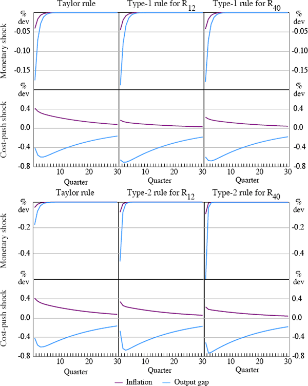
Figures 3 illustrates the impulse responses of inflation and the output gap to a monetary shock and a cost-push shock for a standard Taylor rule, and for type-1 and type-2 rules involving R₁₂ and R₄₀ respectively. The parameters remain fixed across rules in order to capture the effects implied by the maturity dimension of the problem.

A number of interesting features arise from this comparison. First, the signs of the responses do not change across policies. The qualitative responses of inflation and the output gap are the same as those generated by a standard Taylor rule. A contractionary monetary policy shock reduces both inflation and the output gap for all rules considered, while an adverse cost-push shock increases inflation and decreases output for all rules as well. These results suggest that type-1 and type-2 rules do not imply ‘strange’ responses to the disturbances that hit the economy. Secondly, observe that the size of the responses is significantly affected by the type of policy rule. In the case of type-1 rules, in response to a cost-push shock, inflation deviates less than in the Taylor rule case while output suffers a bigger contraction. A similar result shows up in the case of type-2 rules in response to an adverse cost-push shock. In this case, the maturity length of the interest rate in the type-2 rule matters for the determination of the trade-off between output and inflation deviations from the steady state.

Finally, Figure 3 shows that a contractionary monetary shock implies a bigger contraction for inflation and output the longer the maturity of the interest rate in the rule. This arises because the size of the monetary shock changes across policy rules. That is, a one-standard deviation of b_t attached to a type-2 rule for R₄₀ raises the one-period nominal interest rate by more than a one-standard deviation of b_t in a standard Taylor rule. Hence, the size of the monetary policy shock, µ_b, is set to zero in all policy rules for the normative analysis of Section 4.^[19]

As shown, the impulse responses suggest that the dynamic behaviour of the economy is significantly affected by the choice of policy rule. In fact, different rules imply a distinct trade-off between inflation and output deviations in response to a cost-push shock. This shock plays a key role in the conduct of monetary policy. It presents the monetary authority with a trade-off between output and inflation stabilisation. The fact that quantitatively different responses are observed under different rules motivates the question of what is the preferred monetary policy rule. The next section addresses this question.

Footnotes

When monetary policy uses a Taylor rule that involves interest rate smoothing, then the interest rate is a pre-determined variable, inflation and output are jump (or non-pre-determined) variables, and shocks are the exogenous variables. [11]

See Blanchard and Kahn (1980) for a detailed presentation. [12]

Figure 1 shows regions of uniqueness for R₄, R₁₂, R₂₀, and R₄₀. Kulish (2005) contains figures for R₂ as well. [13]

It can be shown in the context of the standard case (that is, with a policy rule of the form
R_1,t = τR_1,t−1 + απ_t + δx_t)
that under the proposed calibration of the model (in particular, λ = 0.14 and α > 1), there are multiple equilibria so long as δ < 0. [14]

See Bernanke and Woodford (1997) for a formal description of a ‘sunspot’ equilibrium. See also Woodford (2003, chapter 4). [15]

McGough et al (2005) also found regions of uniqueness for similar rules in an environment of the same kind. [16]

An earlier version of Kulish (2005) contains figures in α − τ space that illustrate this result. [17]

Variables are expressed in percentage deviations from the steady state. So, in a stationary equilibrium the current expectation of a variable that is far into the future would be zero. [18]

This guarantees that the comparison between policy rules is fair in the sense of capturing only the impact of the deterministic component of the rules. [19]