RDP 2006-11: Component-smoothed Inflation: Estimating the Persistent Component of Inflation in Real Time 4. Results
December 2006
- Download the Paper 313KB
4.1 Australia
Reflecting the fact that Australia has a quarterly CPI, we calibrate Rit for
each series as the variance of its deviations from a 5-quarter Henderson trend. In general, a
5-term Henderson trend removes at least 80 per cent of cycles less than 2.4 periods, so that
deviations of a series from its 5-term Henderson trend should be a good measure of the amount of
high-frequency volatility that we wish to smooth out (ABS 2006). Q is chosen to be 0.5
percentage points, which gives a relatively smooth profile to our measure of underlying
inflation. The parameter β is set equal to 0.15, ensuring that shocks to even the
most volatile series have a half-life no greater than 5 periods, and the parameter  is
set equal to 0.3. We start our sample in 1982, when the ABS introduced the 10th
series of the CPI, so that the first readings for our underlying inflation measure are in 1985.
We also use seasonally adjusted price series where appropriate.[9]
is
set equal to 0.3. We start our sample in 1982, when the ABS introduced the 10th
series of the CPI, so that the first readings for our underlying inflation measure are in 1985.
We also use seasonally adjusted price series where appropriate.[9]
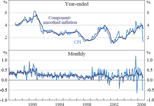
The component-smoothed inflation measure of underlying inflation is shown in Figure 1.[10] It clearly removes much of the volatility in CPI inflation, while still capturing its medium-term trends. Furthermore, despite the smoothing, the peak correlation between component-smoothed inflation and CPI inflation is contemporaneous and many of the peaks and troughs in the measure line up with those of the CPI.
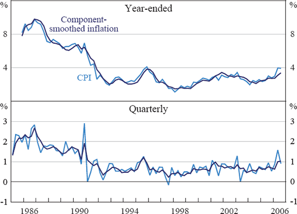
Note: Both series exclude interest charges, major health policy changes and the tax changes of 1999–2000.
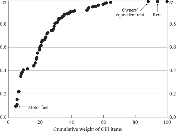
The amount of smoothing applied to each CPI series by our measure can be seen in Figure 2. Our method imposes small α coefficients for the most volatile series, such as fruit, vegetables and automotive fuel, but as Figure 2 indicates, the majority of series have high α coefficients, ensuring that price changes in series with relatively low volatility are quickly incorporated into our measure of underlying inflation. For example, rent has an α coefficient very close to unity, so that price changes in this series are almost immediately incorporated into our component-smoothed inflation measure. Appendix A contains a table reporting the CPI items with the highest and lowest dozen α coefficients.
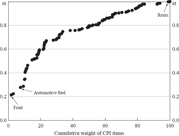
Note: α coefficients and effective weights are for 2006:Q3.
Table 1 indicates how the component-smoothed inflation measure, and a number of commonly used underlying inflation measures, perform on several of the metrics by which underlying inflation series are typically assessed.[11] We present results for the full sample of data, which includes a significant mean shift, as well as over the low-inflation period beginning in 1993. By construction, our measure has a high autocorrelation, especially compared to existing underlying inflation measures over the low-inflation period. Consistent with this, the mean absolute difference of quarterly inflation based on our measure is low, and its standard deviation is lower than that for the headline and exclusion-based measures, and comparable to that for the statistical measures. The component-smoothed inflation measure also tracks trend inflation more closely than the other inflation measures. The measure of trend inflation we have used to assess this is the inflation rate calculated from a centred 9-term Henderson trend of the CPI. Unlike the other measures of underlying inflation, the component-smoothed inflation measure is exactly unbiased relative to the CPI by construction but, as shown in Table 1, unbiasedness is not ensured over any finite sample. Nevertheless, over the full sample of data, the bias is negligible and compares favourably with the exclusion-based and statistical measures. For the low-inflation period since 1993, the point estimate of the bias is slightly smaller than for the trimmed mean, though neither is statistically significant.
| Component-smoothed inflation(b,c) | CPI(b) | CPI ex volatiles | 15 per cent trimmed mean(c) | Weighted median(c) | |
|---|---|---|---|---|---|
| 1985:Q1–2006:Q3 | |||||
| AR(1) coefficient | 0.92 | 0.61 | 0.83 | 0.89 | 0.91 |
| Standard deviation | 0.59 | 0.66 | 0.63 | 0.57 | 0.58 |
| Mean absolute difference | 0.16 | 0.39 | 0.24 | 0.18 | 0.18 |
| Deviation from trend(d) | 0.15 | 0.32 | 0.22 | 0.16 | 0.17 |
| Bias(e) | −0.03 | – | −0.08 | −0.12 | −0.15 |
| 1993:Q1–2006:Q3 | |||||
| AR(1) coefficient | 0.71 | 0.08 | 0.42 | 0.36 | 0.32 |
| Standard deviation | 0.19 | 0.30 | 0.23 | 0.16 | 0.17 |
| Mean absolute difference | 0.11 | 0.31 | 0.18 | 0.14 | 0.16 |
| Deviation from trend(d) | 0.10 | 0.22 | 0.17 | 0.13 | 0.17 |
| Bias(e) | −0.07 | – | −0.19 | −0.10 | −0.13 |
|
Notes: (a) Excluding interest charges and adjusted for the tax changes of 1999–2000. |
|||||
Another common benchmark used to assess measures of underlying inflation is their ability to forecast changes in headline inflation. While the component-smoothed inflation measure is not primarily intended to be used for forecasting, the removal of variability in headline inflation that is likely to be quickly reversed should allow it to perform well as a predictor of headline inflation over short horizons. To assess this, Table 2 reports RMSE statistics when the most recent quarterly inflation rate is used to forecast quarterly headline inflation rates at horizons out to one year. Clearly, all the measures of underlying inflation reported in Table 2 are better predictors of headline inflation at short horizons than headline inflation itself, with the component-smoothed inflation measure performing comparatively well on this criterion.
| Forecast horizon | Component-smoothed inflation(b,c) | CPI(b) | CPI ex volatiles | 15 per cent trimmed mean(c) | Weighted median(c) |
|---|---|---|---|---|---|
| 1985:Q1–2006:Q3 | |||||
| 1Q | 0.47 | 0.58 | 0.50 | 0.43 | 0.42 |
| 2Q | 0.44 | 0.56 | 0.48 | 0.43 | 0.41 |
| 4Q | 0.47 | 0.52 | 0.49 | 0.44 | 0.44 |
| 1993:Q1–2006:Q3 | |||||
| 1Q | 0.33 | 0.41 | 0.37 | 0.32 | 0.33 |
| 2Q | 0.32 | 0.40 | 0.38 | 0.34 | 0.33 |
| 4Q | 0.35 | 0.38 | 0.39 | 0.34 | 0.35 |
|
Notes: (a) Excluding interest charges and adjusted for the tax changes of 1999–2000. (b) Excluding major health policy changes. (c) Based on prices seasonally adjusted at the component level where appropriate. |
|||||
A corollary of good forecasting performance is that divergences between headline inflation and the component-smoothed inflation measure are closed by headline inflation moving towards component-smoothed inflation, rather than the reverse. To test this, we performed pair-wise Granger causality tests between the CPI and the component-smoothed inflation measure, as well as the other underlying inflation measures.[12] The results presented in Table 3 indicate that over the full sample of data, divergences between CPI and underlying inflation are closed by CPI inflation moving towards underlying inflation, and not the reverse (except for the trimmed mean measure). Over the low-inflation period beginning in 1993, there is no statistically significant Granger causality between CPI inflation and any of the underlying inflation measures. This is consistent with the finding in Heath, Roberts and Bulman (2004) that inflation in Australia has become harder to forecast in the low-inflation period.[13]
| 1985:Q1–2006:Q3 Null hypothesis |
1993:Q1–2006:Q3 Null hypothesis |
||||
|---|---|---|---|---|---|
| CPI does not Granger cause candidate series | Candidate series does not Granger cause CPI | CPI does not Granger cause candidate series | Candidate series does not Granger cause CPI | ||
| Component-smoothed inflation(a,b,c) |
0.46 (0.50) |
24.23 (0.00)*** |
|
1.25 (0.27) |
0.98 (0.33) |
| CPI ex volatiles(a) |
0.41 (0.52) |
20.95 (0.00)*** |
|
0.33 (0.57) |
0.53 (0.47) |
| 15 per cent trimmed mean(a,c) |
10.36 (0.00)*** |
53.01 (0.00)*** |
|
0.02 (0.89) |
2.53 (0.12) |
| Weighted median(a,c) |
2.42 (0.12) |
56.34 (0.00)*** |
|
0.28 (0.60) |
1.14 (0.29) |
|
Notes: ***, ** and * denote rejection of the null hypothesis at the 1, 5 and 10
per cent levels of significance; p-values in parentheses below
F-statistics. |
|||||
4.1.1 Relation to other underlying inflation measures
In order to better understand differences between component-smoothed inflation and other measures of underlying inflation, it is helpful to consider the effective smoothing that is applied to each CPI component under the alternative measures. As noted earlier, our measure would be the same as the CPI if αit =1 for all components. Similarly, the CPI ex volatiles is equivalent to a measure with αit =1 for all the included components and αit = 0 for the excluded components (fruit, vegetables and automotive fuel). The items included in the trimmed mean vary from quarter to quarter, but we can get a sense of the amount of volatility in each CPI component, as assessed by the trimmed mean, by calculating the proportion of time each item is included in the trimmed mean. In general, we would expect that series with low α coefficients (those containing a lot of temporary shocks) would be frequently excluded from the trimmed mean, and vice versa.
To show this graphically, Figure 3 updates Figure 2 to include the proportion of time each CPI item has been included in the trimmed mean over the history of each price series.
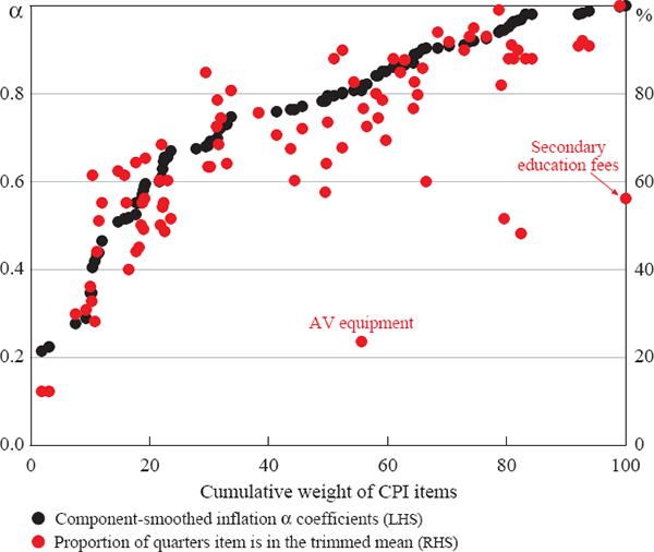
Notes: α coefficients and effective weights are for 2006:Q3. Data for the 15 per cent trimmed mean reflect the proportion of time that items in the 15th series CPI have been in the 15 per cent trimmed mean for each quarter the series has been in existence, except for the deposit & loan facilities and other financial services series, which have only been published since 2005:Q3.
As expected, there is a fairly close correspondence between the α coefficients of each CPI component for our measure and the proportion of time each component has been excluded from the trimmed mean. A notable exception is the series for audio, visual & computing equipment. It is relatively persistent, but is regularly excluded from the trimmed mean. This is because it has experienced a substantial relative price decline. Similarly, secondary education, which is found to be the most persistent series using our method, is regularly excluded from the trimmed mean because it is experiencing a substantial relative price increase, growing at 6.7 per cent per annum on average. At an aggregate level, these offsetting effects seem to cancel out such that the trimmed mean is not significantly biased with respect to headline inflation. Nonetheless, this does suggest some efficiency loss in the trimmed mean compared with the component-smoothed inflation measure as informative movements in audio, visual & computing equipment and secondary education prices are commonly trimmed.
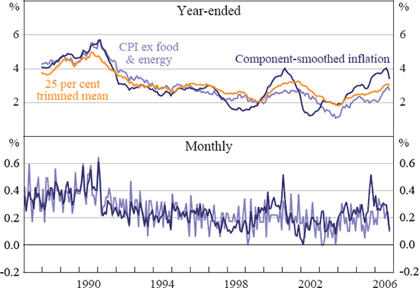
The result of these differences can be seen in Figure 4, which shows year-ended inflation for the component-smoothed inflation measure, the CPI ex volatiles series and the trimmed mean. While these measures all present a broadly similar picture of underlying inflation over our sample, there are some notable differences. In the period between 1995 and 1997 the component-smoothed inflation measure corresponds more closely to the CPI ex volatiles measure than the trimmed mean, which showed a smaller rise in inflation, most likely due to the increase in the positive skewness of CPI inflation over this period. More recently, the component-smoothed inflation measure has diverged from the CPI ex volatiles measure, due in part to the different treatment of automotive fuel. Over the past three years, rises in automotive fuel prices have accounted for around 15 per cent of the rise in the level of our index, and by definition have made no contribution to growth in the CPI ex volatiles measure. Over this same period, automotive fuel prices have only been in the trimmed mean once, though, for reasons mentioned above, they still influence it.
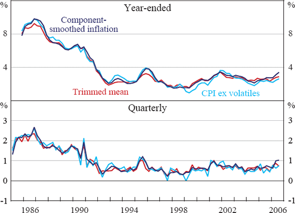
Notes: All series exclude interest charges, and are adjusted for the tax changes of 1999–2000. The componentsmoothed inflation measure has also been adjusted for major health policy changes.
4.2 The United States
Reflecting the monthly frequency of the US CPI, we use different parameters than those used with
the quarterly Australian data. We use a 23-month Henderson trend to calibrate Rit
compared with the 5-quarter Henderson trend used for the Australian data. The 5- and 23-term
Henderson trend series remove the majority of variation in data series at frequencies of less
than 2.4 and 8 periods respectively, and so are comparable measures of noise when used on
quarterly and monthly data (ABS 2006). The parameter Q does not need rescaling because
values for Rit calculated based on a 23-month Henderson trend are broadly
comparable in magnitude to those calculated with a 5-quarter Henderson trend. However, the
parameters and β are scaled down by a factor of
one-third. With these adjustments, the performance of the component-smoothed inflation measure
on US data is similar to that on the Australian data.
Our sample is from 1987:M1 to 2006:M10. Over this period there have been several re-weightings of the US CPI, but only in 1997 were there changes to the items included in the CPI price indices. We use data at the expenditure class level (which currently consists of 70 categories), and are able to obtain data for the bulk of the post-1997 price indices for several years before 1997, allowing us to calculate α coefficients for these series, and so avoiding any break in our underlying inflation measure. For series where data before 1997 are not available, they are assigned the α coefficient of the most similar superseded series for the first three years.
Figure 5 below shows the US CPI and the component-smoothed inflation measure in monthly and year-ended percentage change form. Clearly, our measure of underlying inflation is smoother than headline inflation, particularly in monthly terms. The peak correlation with headline inflation is contemporaneous. As will be seen when this measure is compared with the core measure (CPI ex food & energy) the apparent lag around the turn of the century is induced by large swings in energy prices that turned out to be quite persistent. Of course, at the time this could not be predicted and the delayed response evident in our measure is generally the best one can do in real time.
Notes: The CPI series is the seasonally adjusted series published by the Bureau of Labor Statistics (BLS). The component-smoothed inflation series uses component data that have been seasonally adjusted using Census X12 where appropriate.
The properties of the component-smoothed inflation measure that can be seen in Figure 5 are also evident in the statistics presented in Table 4: relative to the CPI, our measure has high persistence, a low standard deviation and small mean-absolute difference of percentage changes. The bias for the component-smoothed inflation measure is also small over our sample period. The component-smoothed inflation measure is also a smoother measure of inflation than the CPI excluding food & energy (which is the most commonly quoted core CPI measure in the US). Our underlying inflation measure also follows trend inflation more closely than the CPI ex food & energy. For the US, we measure trend inflation as the inflation rate calculated from a centred 23-term Henderson trend of the CPI.
| Component-smoothed inflation(a) |
CPI(b) | CPI ex food & energy(b) | |
|---|---|---|---|
| AR(1) coefficient | 0.78 | 0.29 | 0.39 |
| Standard deviation | 0.11 | 0.22 | 0.12 |
| Mean absolute difference | 0.05 | 0.19 | 0.11 |
| Deviation from trend(c) | 0.06 | 0.18 | 0.11 |
| Bias(d) | 0.02 | – | −0.07 |
|
Notes: (a) Price series have been seasonally adjusted using Census X12 where
appropriate. |
|||
As shown in Figure 6, the distribution of α coefficients for the US is similar to that for Australia. The ranking among CPI item types is also broadly similar. For example, the rent series have α coefficients close to unity, while motor vehicle fuel has a small α coefficient for Australian and US data. Interestingly, even with monthly data, which we might expect to be more noisy than quarterly data, over half the CPI items by weight have an α coefficient of 0.9 or greater, so that price data for at least half the CPI are incorporated rapidly into the component-smoothed inflation measure. See Appendix A for a list of the CPI components with the highest and lowest dozen α coefficients.
Note: α coefficients and effective weights are for 2006:M10.
For brevity, we have not reported the results contained in Table 2 for US data, as the same general conclusions made earlier with Australian data also hold with US data. In particular, the current level of monthly component-smoothed inflation is a better predictor of the future level of CPI inflation at short horizons than the current level of the CPI ex food & energy measure. However, we find that while the component-smoothed inflation measure Granger causes the CPI, the CPI also Granger causes the component-smoothed inflation in a test containing at least two lags.[14]
4.2.1 Relation to other underlying inflation measures
Figure 7 shows the component-smoothed inflation measure and the CPI ex food & energy, together with the 25 per cent trimmed mean series calculated by Brischetto and Richards (2006) in year-ended form. The component-smoothed inflation measure and the core CPI (that is, ex food & energy series) have at times presented quite different indications on the pace of underlying inflation.
Note: The CPI ex food & energy series is the seasonally adjusted series published by the BLS. The componentsmoothed inflation series uses component data that have been seasonally adjusted using Census X12 where appropriate.
Of particular note is the recent divergence created by the increase in oil prices – the component-smoothed inflation measure has been rising since 2004 in year-ended terms while the core measure has only recently kicked up above 2.5 per cent. The component-smoothed inflation measure also indicated more strength in underlying inflation in the late 1990s, and suggested that underlying inflation declined more rapidly than the CPI ex food & energy measure in the early 2000s.
Our measure appears to lead the core CPI measure – particularly through the period around the turn of the century – while it appeared to lag headline during this period (Figure 5). This pattern is consistent with the hypothesis that sustained energy price shocks ultimately lead to inflationary pressures. Whether or not this is the case, our measure can provide an indicator of building price pressures associated with sustained energy price movements in a timely fashion while not providing false signals associated with temporary shocks. This different perspective on such shocks seems potentially useful when combined with evaluations based on other underlying inflation measures. Because energy prices are volatile, and so are typically removed from trimmed mean measures of inflation, the 25 per cent trimmed mean shown in Figure 7 appears also to have excluded most of the first-round effect of higher energy prices in recent years.
Another way to better understand the divergences between the component-smoothed inflation measure and the CPI ex food & energy measure is shown in Figure 8. Figure 8 adds the equivalent α coefficients for the CPI ex food & energy measure to the α coefficients for the component-smoothed inflation measure shown in Figure 6.
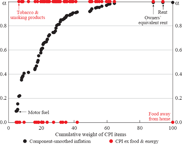
Note: α coefficients and effective weights are for 2006:M10.
Interestingly, the core CPI (which excludes food & energy) removes many items that have relatively high α coefficients, most notably the item food away from home which, based on our measure, we find to be the CPI item containing the least noise.[15] In contrast, the core CPI includes a number of items that we find to be highly volatile, such as tobacco & smoking products. This suggests some efficiency loss for the CPI ex food & energy series by excluding some potentially informative series while including a number of series with similar volatility to other excluded series.
4.3 Sensitivity
Along the way, we have chosen a number of parameter values that affect the performance of the component-smoothed inflation measure. In this section, we discuss the effect of varying these parameters on the component-smoothed inflation measure.
The parameter Q, which controls the variance of the smoothed price series, tends to have little effect on the amount of smoothing that is applied to series containing little noise, but has a larger effect on the amount of smoothing applied to more noisy series. This is because series such as rent have values for Rit which are much smaller than Q, so that αit is close to unity for a wide range of values for Q, but for noisy series such as automotive fuel, Rit is closer to the value of Q we have chosen, so that changing Q has a larger effect on αit for these series. To illustrate this, Figure 9 shows α coefficients for Australian data when Q is three times and one-third the value we have chosen for the component-smoothed inflation measure presented earlier.
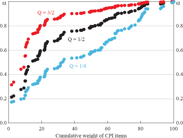
Note: α coefficients and effective weights are for 2006:Q3.
Figure 9 shows that increasing the value of Q has the effect of increasing the α coefficients for each series, but with the largest proportional increase for the most noisy series, and vice versa. In order to gauge the effect of these changes in α parameters on our measure of underling inflation, Figure 10 shows the component-smoothed inflation measure in year-ended percentage change form for Australia and the US when Q is scaled to be one-third and three times the value we have chosen.
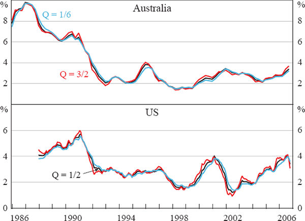
As expected, higher values of Q, which reduce the amount of smoothing applied to CPI series, result in a more variable component-smoothed inflation measure, more closely following CPI inflation. However, the differences are not substantial, despite the wide range of parameter values we have shown; for both Australia and the US, the component-smoothed inflation presents a broadly similar picture of underlying inflation for each of the three values of Q shown in Figure 10.
The method we have chosen to assess the amount of volatility in each price series, namely the variance of deviations of price series from their Henderson trend, can be replaced with a variety of other methods. For example, using the mean-squared difference or variance of percentage changes in each price series produces a similar ranking of relative noise content of CPI items. As mentioned earlier, the magnitude of Rit is not important because Q is chosen relative to Rit and the resulting component-smoothed inflation measures are similar to the ones presented in this paper.
Using the autoregressive parameter from a simple regression of a price series on its own lag is, despite its superficial appeal, an inferior approach. The problem is that it does not distinguish between short- and medium- or long-term trends. Thus, over a period of significant disinflation where there is a large change in the mean level of inflation, most series will have a high autoregressive parameter regardless of the amount of temporary volatility in the series. Even absent a mean shift in the general level there are still problems with using the autoregressive parameter. To illustrate this, Figure 11 below plots the autoregressive parameter for each item in the Australian CPI calculated over the low-inflation period against the α we choose based on deviations from the Henderson trend. Significant deviations from a straight line indicate that the measures are not close substitutes. As can be seen, there is little correlation between the measures and many of the autoregressive parameters are actually negative, which complicates interpretation further.
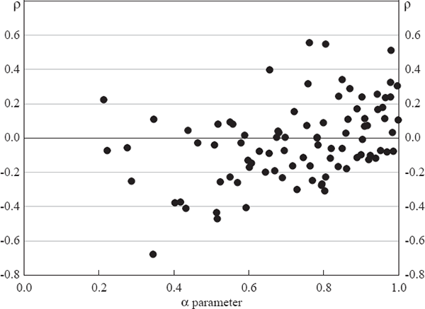
Note: Autoregressive parameters calculated over the low-inflation period 1993:Q1–2006:Q3.
Footnotes
We use the same seasonal adjustment as is used for the 15 per cent trimmed mean measure used by the Reserve Bank of Australia (RBA). The seasonal adjustment process is discussed in more detail in Roberts (2005). [9]
The temporary shock to banana prices in Australia in the June and September quarters of 2006 is having some effect on the level of underlying inflation shown by our component-smoothed inflation measure. Because we know this shock will be temporary, we can use this knowledge to set α = 0 for the fruit price series in the June and September quarters 2006, ensuring that our measure does not update in response to the surge in banana prices. Adjusting for banana prices in this way has the effect of reducing the inflation rate for the component-smoothed inflation measure from 3.4 to 3.2 per cent over the year to the September quarter 2006. [10]
We use the 15 per cent trimmed mean for comparison because that trim is the one currently published by the RBA. Work by Brischetto and Richards (2006) examines the full range of possible trimmed means and finds that the performance of trimmed means are very similar for trims greater than, approximately, 5–10 per cent. [11]
Roberts (2005) outlines a number of other tests that address this property. [12]
Brischetto and Richards (2006) discuss the use of Granger causality tests in more detail and suggest some caution when interpreting the results. [13]
Brischetto and Richards (2006) presents a wider range of Granger causality tests for the US. [14]
Clark (2001) also finds the CPI item food away from home to be highly persistent. [15]