RDP 2007-09: Private Business Investment in Australia Appendix B: Chain-linking and Investment
September 2007
- Download the Paper 467KB
The real investment and capital stock data used in this paper are constructed by the ABS using a chain-linking approach. Formally, these series are chained Laspeyres volume indices. Chain-linking is used because it arguably produces better estimates of real growth rates, but problems exist with chain-linked levels estimates. In particular, the real levels estimates may suffer from ‘non-additivity’ – that is, aggregates will not necessarily be equal to the sum of their components. This non-additivity means that levels estimates many years ago may not have an intuitive interpretation – a point raised in Section 2.2.1. Non-additivity tends to become particularly significant where there have been large relative price shifts between the components of a series. For Australian investment data, large relative price shifts are evident in computing equipment and livestock investment, thereby creating problems for investment series that include these components (Table B1).
| Relative investment prices | Number of times relative prices have halved between 1985/86 and 2005/06 |
|||
|---|---|---|---|---|
| 1965/66 | 1985/86 | 2005/06 | ||
| Computing equipment | 100.0 | 1.1 | 0.02 | 30.9 |
| Computer software | 100.0 | 65.0 | 16.9 | 1.9 |
| Livestock | 100.0 | 24.3 | 19.6 | 0.6 |
| Business investment | 100.0 | 82.6 | 52.2 | 0.8 |
| Business investment excluding computing equipment | 100.0 | 90.1 | 78.7 | 0.6 |
| Business investment excluding computing equipment & livestock | 100.0 | 104.8 | 92.8 | 0.6 |
|
Sources: ABS, authors' calculations |
||||
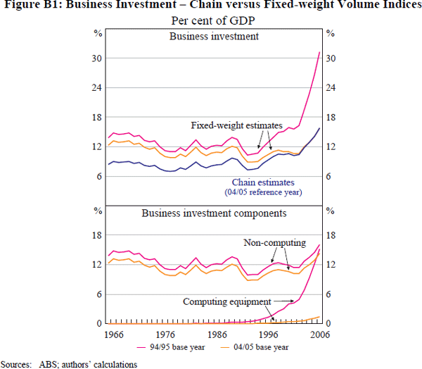
Some of the advantages and disadvantages of chain-linking can be illustrated by a comparison with alternative fixed-weight estimates. Additivity always holds for fixed-weight indices (by definition), but relative price changes mean that the weight of sub-components (such as computing) can vary substantially with different base years. This means that the level of investment can change significantly if a different base year is chosen (Figure B1, top panel). Chain-linked series do not face this problem (an advantage) as their growth rate is a compromise between fixed-weight series with different base years. This reflects the fact that the chain series allows the weight given to the components to vary over time.

The loss of additivity of chain-linked series (a disadvantage) is evident in Figure B1 (bottom panel) as the sum of the non-computing and computing components of investment do not add to the chain estimates in the top panel. Also, the level of the aggregate chain series is difficult to interpret, being not only below the two fixed-weight estimates but also below the series for just non-computing investment for most of the sample (top versus bottom panels).
B.1 Depreciation Rates
In this paper, we solve most additivity problems by removing computing from investment and depreciation. In part, this is important because non-additivity can greatly distort measures of depreciation rates in ways discussed below.
Many investment models make use of the capital accumulation identity (as in Equation (B1)) and assume that the depreciation rate can be treated as a constant. However, because of non-additivity, the capital accumulation identity need not hold in practice and therefore the assumption of a constant depreciation rate might be flawed when the model is taken to the data. As such, the capital accumulation identity should be not be used for deriving depreciation rates, as illustrated by Tevlin and Whelan (2003) using US data.
Instead, depreciation rates at their most disaggregated level should be measured by taking the ratio of the consumption of fixed capital (COFC, otherwise known as depreciation) during a period to the stock of capital at the beginning of the period, as follows:
However, non-additivity means that aggregate measures of depreciation (as calculated by Equation (B2) at the aggregate level) are not necessarily a weighted average of the depreciation rates of their sub-components. If non-additivity exists, then the average depreciation rate calculated in this way may have weights on subcomponents that do not sum to one. As such, a correction is needed to force the weights to sum to one.
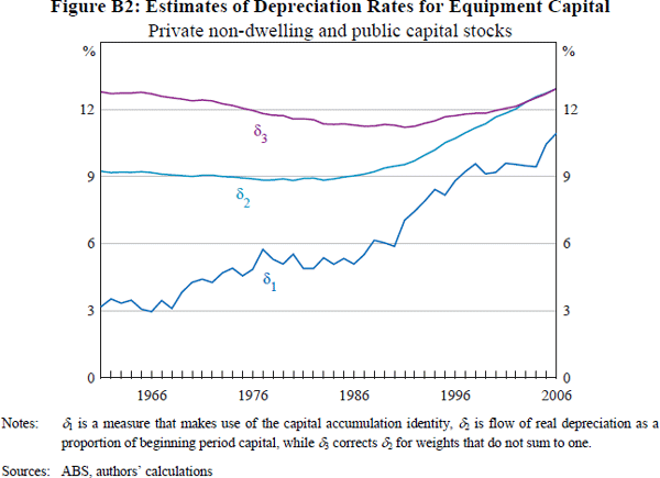
The differences between these possible measures are illustrated in Figure B2 for equipment capital (including computing). δ1 is measured indirectly using the capital accumulation identity (Equation (B1)). δ2 is the depreciation rate constructed in the fairly standard fashion of taking the ratio of depreciation of equipment capital during the period to the capital stock at the beginning of the period as in Equation (B2). δ3 is also based on Equation (B2) (but at a disaggregated level) and includes the correction to weight the depreciation rates of the components with weights that sum to one. The difference between the measures is stark, and highlights the importance of calculating depreciation rates correctly.


