RDP 2007-09: Private Business Investment in Australia 4. Results
September 2007
- Download the Paper 467KB
4.1 The Traditional Neoclassical Long Run
The relationship between the capital-to-output ratio and the cost of capital suggested by the traditional neoclassical model is estimated separately for non-computing equipment and structures capital.[10] The exact specification is based on taking the natural log of Equation (1) and transforming it so that the dependant variable is (k − y) (that is, the log difference between the real capital stock and real GDP). Structures capital is not split further into the engineering and buildings sub-components owing to data limitations. The cost of capital (also logged, ct) is measured as described by Equation (2). With some evidence that most of the series are non-stationary (see Appendix C), these long-run relationships are modelled using cointegration techniques. Table 1 shows regression results using both OLS and DOLS, the latter being recommended by Caballero (1994) who shows that the coefficient on the cost of capital is biased towards zero when OLS is used.[11]
| Equipment (excluding computing) | Structures | ||||
|---|---|---|---|---|---|
| OLS | DOLS | OLS | DOLS | ||
| Cost of capital (ct) | 0.23*** (0.05) |
0.63*** (0.08) |
0.12** (0.06) |
0.34*** (0.06) |
|
| Number of leads | 0 | 10 | 0 | 10 | |
| Number of lags | 0 | 20 | 0 | 20 | |
| Cointegration tests: | |||||
| ADF | −1.90 | −1.89 | −0.77 | −4.13*** | |
| Notes: ***, ** and * denote significance at the 1, 5 and 10 per cent levels respectively. Newey-West corrected standard errors are in parentheses. All variables are in logs. Data available until 2006:Q2, with earlier end-date allowing for leads in the DOLS regressions. ADF denotes Augmented Dickey-Fuller tests which have a null hypothesis of no cointegration. Results are compared with MacKinnon (1991) tables. | |||||
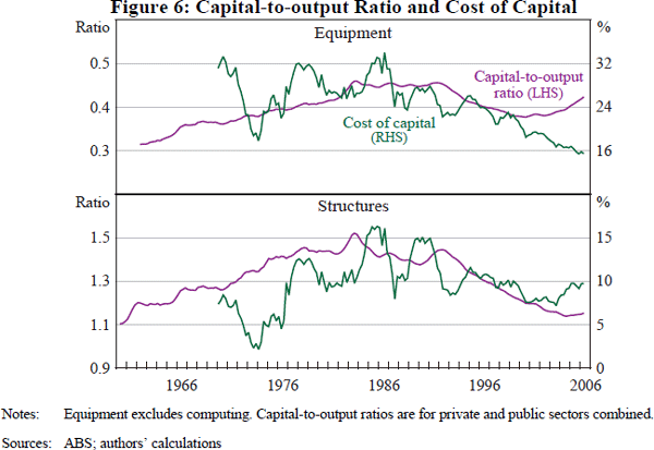
In contrast to theory, the results suggest a positive relationship between the capital-to-output ratio and the cost of capital across all models,[12] although for aggregate investment most models do not appear to be cointegrated, with the exception of the DOLS model for structures. An inverse relationship is apparent only in a few brief periods, with the capital-to-output ratio and the cost of capital otherwise positively related (Figure 6). One possible explanation for the positive coefficient is that the models are tracing out a relatively fixed upward-sloping supply curve for capital, rather than the downward-sloping demand curve; the latter being subject to substantial fluctuations as firms respond to changing expectations about the future profitability of investment (see Schaller 2006). An alternative explanation is that the capital stock is poorly measured, leading to biases in the estimation of the traditional neoclassical long run. Difficulties in finding an inverse relationship for aggregate investment are not uncommon in the literature.
4.2 An Alternative Neoclassical Model
Another approach, which is adopted below and is commonly used in the literature, is to modify the traditional model so as to look for an inverse relationship between the investment-to-output ratio and the cost of capital (see, for example, Bean 1981, Bakhshi et al 2003 and Bond and Hernandez 2003). This transformation is due to Bean and is justified by an approximate relationship that should exist between the capital-to-output ratio and the investment-to-output ratio:
where lower case variables k, i and y are logs of capital, investment and output. This approximation holds as long as growth in the capital stock ( g ) is small relative to the depreciation rate (δ).[13] Furthermore, if movements in δ and g are small relative to changes in i − y and k − y, then a roughly proportionate relationship should exist between the investment-to-output ratio and the capital-to-output ratio. This approach has the advantage that investment may be considered to be measured more reliably than capital, which is not directly observed but rather derived from the former.
Using models based on investment rather than capital allows a further disaggregation of structures investment into building and engineering investment. Unit root tests are presented in Appendix C and suggest either the presence of a unit root or an ambiguous result for investment shares and their respective cost-of-capital measures. To allow for the potential non-stationarity of the series, error-correction models (ECMs) of the following form are estimated:
This formulation places growth in investment as the dependant variable, in contrast to the common alternative of using the investment-to-capital ratio. This is desirable as the investment growth rate is often the variable of interest to macroeconomists. However, it comes at a cost of a more volatile dependant variable, making modelling more difficult.
A vector of short-run variables, Xt, is included to help explain deviations (of the level of investment) from the long-run equilibrium, which are often attributed to frictions that restrict a firm's ability to adjust immediately (such as financial frictions or physical constraints).[14] In the first set of regressions below, Xt includes only lags of investment growth, GDP growth, and changes in the cost of capital (though only from the second year to avoid potential endogeneity) as implied by the standard neoclassical model.[15]
A broader list of factors for Xt is then also investigated, including business confidence, and first differences in the real exchange rate, the terms of trade and Q. These additional variables are intended to make up for some potential difficulties associated with measuring the cost of capital, and to better capture the short-run dynamics. For example, difficulties in measuring the cost of engineering capital might lead to a role for the terms of trade in explaining engineering investment. This arises because output prices for firms undertaking engineering investment (such as mining firms) are approximated by the GDP deflator and are therefore likely to understate the fall in the relative cost of capital in the export-oriented sector when the terms of trade rises.
Lags of real corporate profit growth (as a proxy for cash flows) were also included in the short-run specification in an attempt to control for the possible dynamic impact of financial frictions. These variables are neither statistically nor economically significant (and hence not reported), in contrast to a number of existing studies (including Debelle and Preston 1995 and La Cava 2005). This might be because other investment models use a levels measure of cash flows (as a proportion of the capital stock),[16] which is not as noisy as the growth rate measure tested here.
As before, the cost of capital for equipment and engineering is measured according to Equation (2). For building, however, a term for the expected financial gain from holding capital (EπK,t) is also included as follows:
This is consistent with the original Hall and Jorgenson (1967) formulation, but they assumed expectations to be static. In contrast, Tevlin and Whelan (2003) and Bakhshi et al (2003) model expectations as a moving average of growth in actual relative investment prices over three years and two years respectively. In Australia, expectations of capital gains appear to have been an important driver of building investment (particularly during the late 1980s commercial property boom) and so should be included in the cost of capital. However, the absence of a second-hand market in mines, ports or purpose-built equipment suggests a less important role for capital gains in motivating other types of investment. For this reason, a measure of capital gains is included only for buildings.[17]
Such a measure can be constructed in a similar way to Bakhshi et al (2003) and Tevlin and Whelan (2003), as an 11-quarter-centred moving average of year-ended real office price growth. However, office price growth was so rapid in the late 1980s that the implied building cost of capital becomes negative. This may reflect the omission of prices for other assets in this class of investment (factories or shopping malls for example), as well as the difficulty of capturing investors' true beliefs regarding capital gains from a measure of prices of buildings that sold in a given period. Either way, arbitrage conditions suggest that such extreme movements in office prices would not necessarily be the best measure of expected capital gains or losses.[18] To deal with this, it is assumed that half of people hold these expectations, while the other half expect real office prices to grow at their long-run average rate (which is around zero). The resulting building cost of capital is always positive and peaks much lower during the office market downturn in the early 1990s. The results of the following regressions are qualitatively similar to the alternative (11-quarter moving average) formulation.
As mentioned above, one difficulty in estimating the specification in Equation (4) is the volatility of the dependant variable. The standard deviations of quarterly growth in investment are around 6 percentage points for non-computing equipment and buildings, and around 7½ percentage points for engineering. This compares to around 1 percentage point for quarterly GDP growth. There are two potential problems as a result: the coefficients may not be very precisely estimated, but more worryingly, the coefficient estimates may be susceptible to influential observations.
To combat this problem, the DFFITS outlier testing methodology of Belsley, Kuh and Welsch (1980) is used.[19] For the parsimonious specifications, between 5 and 10 per cent of each sample is found to be influential and is removed from the estimated models.[20] This seems reasonable as some movements may reflect measurement error while others may be difficult to explain with a relatively parsimonious model. Models that excluded the influential observations were found to be more robust to variations in sample periods and specifications than those including all observations.[21]
4.3 Error-correction Model Results
As a prelude to the main results, Table 2 presents the results of the error-correction models based on the narrow form of Xt, which includes only the variables implied by the neoclassical model. For all models, the coefficient on the cost of capital in the long run is negative (although it is not always statistically significant and its size is somewhat sensitive to alternative dynamic specifications (not reported)). An Engle-Granger test implies cointegration between investment shares and the relevant cost of capital for building and engineering investment. Significant t-statistics on the error-correction terms imply cointegration for equipment and engineering investment. The fit of the model is acceptable for building and engineering investment. The rather poor fit for equipment investment reflects the large number of insignificant coefficients in this unrestricted model.
| Equipment (1) 1974–2006 |
Building (2) 1986–2006 |
Engineering (3) 1979–2006 |
|
|---|---|---|---|
| Long run (dependant variable: i−y) | |||
| Cost of capital (c) | −0.46 (−1.57) |
−0.59 (−1.24) |
−1.61 (−3.16) |
| ADF t-statistic(a) | (−2.68) | (−3.44) | (−3.99) |
| Short-run results (dependant variable: Δit) | |||
| Error-correction term | −0.12 (−2.74) |
−0.06 (−1.55) |
−0.10 (−2.67) |
 |
0.15 (0.62) |
0.52 (2.45) |
0.51 (3.71) |
 |
0.36 (1.70) |
−0.07 (−1.05) |
0.30 (2.31) |
 |
0.78 (0.54) |
−0.21 (−0.09) |
3.06 (1.96) |
| Adjusted R-squared | 0.17 | 0.37 | 0.42 |
| Included/total observations | 119/129 | 71/80 | 103/109 |
| Notes: Figures in parentheses are Newey-West t-statistics. Sums
of coefficients and associated t-statistics are reported. Joint
tests on the sum of coefficients are significant at 10 per cent for all
variables except lagged investment in Model 1. (a) The 10 per cent critical value for the Engle-Granger cointegration test is about −3.1 (MacKinnon 1991) |
|||
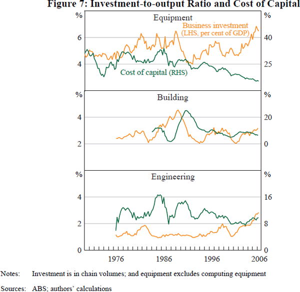
Figure 7 compares investment shares of GDP with the cost of capital for the three types of investment. A loose inverse relationship is apparent for equipment. The relationship is more obvious for building investment during the boom/bust period of the later 1980s and early 1990s. The relationship for engineering is less obvious.
The results based on the broader form of Xt are presented in Tables 3, 4 and 5 for equipment, building and engineering investment respectively. The most parsimonious (and generally preferred) models are displayed on the left of each table. These are restricted forms of the more general models on the right, which are presented to illustrate the robustness of the results. The adjusted R-squared values are reported excluding the identified influential observations, rather than assuming that those observations have been perfectly predicted.
| Parsimonious model (1) | Common (2) | With RER (3) | With GDP (4) | ||||||||
|---|---|---|---|---|---|---|---|---|---|---|---|
| 74–06 | 90–06 | 74–06 | 90–06 | 74–06 | 90–06 | 74–06 | 90–06 | ||||
| Long run (dependant variable: i–y) | |||||||||||
| Cost of capital (c) | −0.60 (−3.25) |
0.22 (0.79) |
−0.77 (−2.52) |
−0.35 (−4.06) |
−0.24 (−2.59) |
||||||
| ADF t-statistic(a) | (−2.61) | (−2.04) | (−2.63) | (−2.13) | (−1.80) | ||||||
| Short-run results (dependant variable: Δit) | |||||||||||
| Error-correction term | −0.14 (−2.94) |
−0.08 (−2.64) |
−0.11 (−2.04) |
−0.26 (−4.35) |
−0.23 (−4.52) |
||||||
| ΔRERt−2 | 0.48 (6.23) |
0.55 (4.62) |
0.53 (7.22) |
0.53 (4.85) |
|||||||
 |
0.02 (0.07) |
1.00 (2.96) |
0.06 (0.23) |
0.86 (3.06) |
|||||||
| Business confidencet−1 | 0.07 (9.87) |
0.04 (4.36) |
0.07 (9.06) |
0.06 (4.65) |
0.06 (6.80) |
0.04 (5.51) |
0.06 (6.11) |
0.05 (3.25) |
|||
| Δct−8 | −0.16 (−2.11) |
−0.17 (−2.33) |
0.00 (0.00) |
−0.17 (−2.34) |
−0.20 (−2.52) |
||||||
| Δit−1 | −0.22 (−3.64) |
−0.18 (−2.85) |
−0.18 (−1.80) |
−0.25 (−3.45) |
−0.25 (−3.34) |
||||||
 |
1.08 (2.44) |
1.69 (2.56) |
1.14 (2.91) |
1.55 (2.33) |
0.84 (2.21) |
1.55 (2.31) |
|||||
 |
−0.48 (−0.45) |
1.75 (1.49) |
|||||||||
 |
0.06 (0.77) |
0.34 (2.86) |
0.11 (1.30) |
0.46 (3.99) |
|||||||
| Adjusted R-squared | 0.43 | 0.39 | 0.49 | 0.42 | 0.48 | 0.59 | 0.46 | 0.67 | |||
| Included/total observations | 123/129 | 63/66 | 121/129 | 62/66 | 117/129 | 59/66 | 118/129 | 55/66 | |||
| Notes: Figures in parentheses are Newey-West t-statistics. Sums
of coefficients and associated t-statistics are reported for multiple
lags. All multiple lags are jointly significant at the 10 per cent level
except Q over the full sample. (a) The 10 per cent critical value for the Engle-Granger cointegration test is about –3.1 (MacKinnon 1991) |
|||||||||||
| Parsimonious model (1) | Including Δct (2) | General (3) | ||||||
|---|---|---|---|---|---|---|---|---|
| 86–06 | 90–06 | 86–06 | 90–06 | 86–06 | 90–06 | |||
| Long run (dependant variable: i−y) | ||||||||
| Cost of capital (c) | −0.65 (−2.02) |
−0.46 (−1.91) |
−0.54 (−1.74) |
−0.23 (−1.11) |
−0.59 (−1.24) |
0.13 (0.62) |
||
| ADF t-statistic(a) | (−3.58) | (−2.69) | (−3.72) | (−2.96) | (−3.44) | (−2.19) | ||
| Short-run results (dependant variable: Δit) | ||||||||
| Error-correction term | −0.06 (−2.10) |
−0.08 (−3.04) |
−0.05 (−1.86) |
−0.09 (−1.58) |
−0.06 (−1.55) |
−0.11 (−1.99) |
||
| Δit−2 | 0.26 (2.94) |
0.30 (3.02) |
0.22 (2.19) |
0.33 (3.92) |
||||
 |
0.52 (2.45) |
0.77 (3.25) |
||||||
 |
−0.09 (−1.77) |
−0.04 (−0.41) |
−0.07 (−1.05) |
−0.08 (−0.91) |
||||
 |
−0.21 (−0.09) |
1.36 (0.58) |
||||||
| Adjusted R-squared | 0.26 | 0.34 | 0.35 | 0.42 | 0.37 | 0.55 | ||
| Included/total observations | 76/80 | 62/66 | 72/80 | 61/66 | 71/80 | 61/66 | ||
| Notes: Figures in parentheses are Newey-West t-statistics. Sums
of coefficients and associated t-statistics are reported for multiple
lags. All multiple lags are jointly significant at the 10 per cent level. (a) The 10 per cent critical value for the Engle-Granger cointegration test is about −3.1 (MacKinnon 1991) |
||||||||
| Parsimonious model (1) | With RER (2) | With Q (3) | General (4) | ||||||||
|---|---|---|---|---|---|---|---|---|---|---|---|
| 79–06 | 90–06 | 79–06 | 90–06 | 79–06 | 90–06 | 79–06 | 90–06 | ||||
| Long run (dependant variable: i–y) | |||||||||||
| Cost of capital (c) | −0.83 (−5.07) |
−0.81 (−3.62) |
−0.61 (−4.63) |
−0.74 (−3.70) |
−0.70 (−4.18) |
−0.78 (−4.26) |
−0.81 (−4.17) |
−1.01 (−2.78) |
|||
| ADF t-statistic(a) | (−3.57) | (−2.70) | (−2.15) | (−1.46) | (−3.37) | (−2.66) | (−3.54) | (−2.96) | |||
| Short-run results (dependant variable: Δit) | |||||||||||
| Error-correction term | −0.15 (−5.60) |
−0.15 (−5.38) |
−0.17 (−5.87) |
−0.19 (−7.38) |
−0.15 (−4.66) |
−0.18 (−6.54) |
−0.13 (−5.24) |
−0.15 (−5.63) |
|||
 |
0.57 (5.49) |
0.48 (3.58) |
0.76 (7.36) |
0.77 (5.04) |
0.70 (6.28) |
0.79 (5.33) |
0.66 (5.87) |
0.70 (4.93) |
|||
 |
2.59 (6.04) |
3.52 (7.82) |
2.76 (6.50) |
3.06 (5.55) |
2.16 (3.99) |
2.31 (4.42) |
2.07 (4.02) |
1.88 (2.39) |
|||
 |
0.09 (0.26) |
1.19 (2.96) |
−0.01 (−0.02) |
0.85 (2.23) |
0.24 (0.59) |
0.92 (2.29) |
|||||
 |
0.13 (2.18) |
0.33 (2.66) |
0.17 (2.72) |
0.21 (1.75) |
|||||||
 |
−0.64 (−0.52) |
−1.65 (−1.07) |
|||||||||
| Adjusted R-squared | 0.44 | 0.48 | 0.57 | 0.60 | 0.56 | 0.69 | 0.66 | 0.69 | |||
| Included/total observations | 99/109 | 61/66 | 100/109 | 64/66 | 101/109 | 61/66 | 97/109 | 57/66 | |||
| Notes: Figures in parentheses are Newey-West t-statistics. Sum
of coefficients and associated t-statistics are reported for multiple
lags. All multiple lags are jointly significant at the 10 per cent level
(except for Q over the shorter sample). (a) The 10 per cent critical value for the Engle-Granger cointegration test is about −3.1 (MacKinnon 1991) |
|||||||||||
For equipment investment (excluding computing equipment, Table 3), cointegration is found only in the shorter sample period (based on t-statistics for the coefficient on the error-correction terms), so the parsimonious specification for the full-sample period includes only variables in difference form (with the exception of business confidence).[22] Nevertheless, for the long sample there is a statistically significant negative relationship between investment and the cost of capital in the short run (Model 1). In the shorter sample, the long-run coefficient on the cost of capital is close to −0.6 and is within the range suggested by international studies (see Ellis and Price 2004 and Barnes, Price and Sebastia-Barriel 2007). Model 2 presents a common formulation for both sample periods. All of the models imply a significant role for the real exchange rate and business confidence in the short-run dynamics. The role for changes in Q is less robust across the specifications. The results with up to eight lags of GDP growth, changes in Q and the real exchange rate (Model 4) suggest possible over-fitting of the data (especially for the shorter sample period, for which the adjusted R-squared value rises substantially). Finally, the fit of the parsimonious equipment model in Table 3 is substantially better than the model presented in Table 2.
For building investment (Table 4), the extra variables of the broader specification for Xt were not found to be significant. The parsimonious Model 1 includes only a cointegrating relationship and a lagged investment term. It provides a reasonable fit of the data given the lack of short-run dynamics, with evidence of a cointegrating relationship (over the full-sample period). The coefficient on the cost of capital is around −0.5 (again consistent with a number of international studies). The speed-of-adjustment coefficient appears relatively modest, though is statistically significant. The long-run coefficient on the cost of capital is similar to that presented in Table 2, though is more significant. Additional lags of the cost of capital, investment growth and GDP growth are often not statistically significant and do not add much to the fit of the regression.
For engineering investment (Table 5), a robust cointegrating relationship is found for all of the specifications and both sample periods (based on the t-statistics on the error-correction coefficient). The long-run coefficient on the cost of capital is not significantly different from −1, the value implied by a Cobb-Douglas production function. The coefficients on the terms of trade are positive and robust across the various specifications. The fit of the models rise substantially as more short-run dynamic terms are added to the specification, but with little change in the long-run relationship or the coefficient on the error-correction term. The fit of the parsimonious model is similar to that of the model in Table 2 (measured by the adjusted R-squared), as is the significance of the cost of capital and error-correction terms (though the estimated coefficient on the cost of capital is somewhat smaller).
The coefficients on the real exchange rate are positive (but less robust), which might seem surprising given the relatively high export orientation of these firms (with an appreciation in the exchange rate reducing export revenue, other things equal). Further, it is unlikely that the exchange rate would reduce the cost of engineering investment because it has a relatively small imported component. Hence, it is likely that the positive coefficient on the real exchange rate reflects multicollinearity between the terms of trade and the real exchange rate.
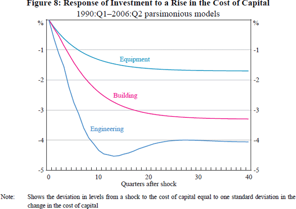
Figure 8 shows the estimated dynamic response of each type of investment to a shock to the level of the respective cost of capital (equivalent to one standard deviation of the change in that cost of capital). These are based on the parsimonious models over the 1990:Q1–2006:Q2 sample.[23] The results illustrate the importance of the cost of capital for engineering investment, reflecting its relatively high long-run coefficient. The role of the cost of capital is also important for building investment, in part due to the fact that a one standard deviation shock to the building cost of capital is relatively large.[24] In contrast, the response of equipment investment to its cost-of-capital term appears relatively modest. The adjustment of equipment and engineering investment towards long-run equilibrium is relatively rapid, compared with the adjustment of building investment.
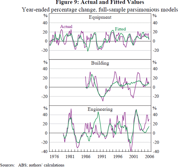
The reasonable fit of the models is shown in Figure 9, which presents year-ended percentage changes in investment along with the implied fitted values for each full-sample regression. Fitted values for the influential observations are calculated as if the general regression results hold for these observations (rather than assuming these observations are perfectly predicted). This leads to some divergences between fitted and actual values, which generally persist for four quarters given the plots are on a year-ended basis. The largest discrepancy seems to be the fall and subsequent recovery in building investment following the Sydney Olympics and the introduction of the GST. Given the one-off nature of these events, such a miss was also unlikely to be captured by standard economic factors. The relatively poor fit of engineering investment in 2005 probably reflects the large amount of road construction undertaken by the private sector on behalf of the public sector. Naturally, the model cannot explain this behaviour.
The variables included to capture the short-run dynamics generally have the expected signs. Notably, for equipment investment, the models identify a powerful role for business confidence across all specifications (Figure 10 shows contributions for the full-sample parsimonious model). Business confidence appears to be capturing broader cyclical factors and taking explanatory power away from other variables.
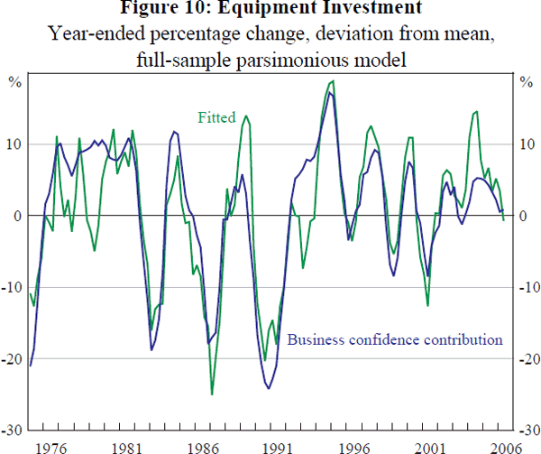
The results also provide some evidence of a positive relationship between the real exchange rate and non-computing equipment investment. This is consistent with the possibility that when the exchange rate appreciates, firms benefit from lower prices of imported equipment, but it is worth noting that an appreciation implies tougher international competition for exporters and import-competing firms (other things equal). The results suggest that the former effect is more important, and tends to have its maximum impact after six months, with evidence of an unwinding of the effect after two years over the full sample.[25]
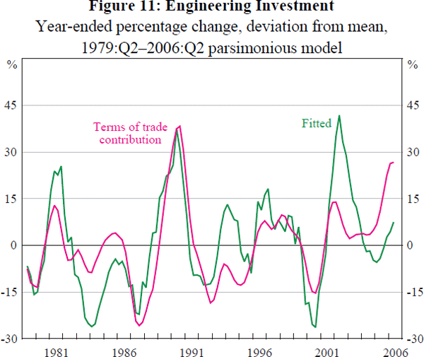
For engineering investment, all specifications identify an important role for the terms of trade in the short run (Figure 11). A 10 per cent increase in the terms of trade is estimated to increase investment by around 25 per cent within eight quarters.[26] There is also a small role for increases in Q.
4.4 Further Robustness Tests
Four further tests of the robustness of the results were examined. First, the parsimonious models for each investment type were estimated including identified influential observations. For equipment, all of the key variables (such as the cost of capital, business confidence and the real exchange rate) are significant at the 1 per cent level, with largely unchanged coefficients. Similarly, key variables in the engineering equation (the cost of capital and the terms of trade), have largely unchanged coefficients and remain highly significant. Over the full sample, the coefficient on the cost of capital in the building equation falls by less than one standard error, and is still significant at the 10 per cent level. This suggests that the main results of the paper are robust to the inclusion of influential observations. Nonetheless, excluding influential observations is important for avoiding spurious relationships when testing various specifications of the model.
Second, in an unrestricted model, with up to 8 lags of each variable in the short-run dynamics, there may be a lack of degrees of freedom and a risk of over-fitting the data. One way around this is to consider regressions with coefficients on adjacent lags of the same variable restricted to be equal (as in Gordon 1997). The key results discussed above are generally robust to these restrictions being placed on lags of GDP, the cost of capital, Q, terms of trade and the real exchange rate.
The third extension was to consider the potential role of the privatisation of former government trading enterprises in driving the estimated relationships for private investment considered in Section 4.3. The reclassification of the investment of these public enterprises might cause the long-run private investment share to trend up during the 1990s, a period of considerable privatisation. To test this, the cumulative value of privatisations as a share of stock market capitalisation can be included as part of the long-run relationships in each of the preferred models. In all models, this variable is statistically insignificant and the size of the estimated coefficients on the cost-of-capital variables did not change substantially.
A fourth extension was to examine results including a time trend in the long-run relationship. As well as being an alternative means of controlling for trends such as privatisation, this could also help to control for possible trends in investment in non-computing equipment (as a share of GDP), in light of the rise in the prominence of computers in a wide range of business activities over this period (which could have led to substitution away from non-computing investment, for example). This inclusion does not affect the size or significance of the cost of capital and error-correction term in the building and engineering models over the full sample, with some of the shorter sample results being less robust. For equipment, the coefficient on the cost of capital is still negative, but smaller and statistically insignificant (reflecting collinearity between the cost of capital and a time trend in the post-1990 sample). Nonetheless, the time trend is statistically insignificant for all models.
Footnotes
Capital stock data are only available for combined public and private sectors. [10]
Using quarterly US data, Caballero (1994) finds a coefficient of −0.4 on the cost of capital when estimated by OLS, but this falls to −0.9 when estimated by DOLS using 25 lags. [11]
These results are in contrast to La Cava (2005), who estimates a coefficient of −0.6 using Australian firm-level data. [12]
This assumption is likely to hold more closely for equipment investment, where the depreciation rate is large. [13]
Also, there may be an option value of waiting if investment is irreversible and future returns are uncertain (Pindyck 1991). [14]
It is possible that a spike in the price of investment goods reflects increased orders of investment goods to be delivered over coming quarters. This would lead investment and the cost of capital to be positively related, as the data trace out the supply curve rather than the demand curve. A simple way of getting around this is to only include longer lags of (changes in) the cost of capital – the approach taken here. The key results are robust to extra lags (long and short) of Δct. [15]
The ratio of cash flows to the capital stock is used in these studies so as to be consistent with the dependant variable (the investment-to-capital ratio). However, the growth rate of cash flows is more likely to explain quarterly investment growth, which is the dependant variable used in this paper. [16]
Even if firms were able to sell their equipment or engineering capital, these assets are so heterogeneous, illiquid and subject to considerable adjustment costs that it is difficult to measure these prices. Cost-of-capital measures that include a measure of financial gain for equipment and engineering were examined and produced broadly similar results. The significance of the cost of capital in the equipment equation, however, was reduced. [17]
If the expected capital gain had been that high, it seems likely that investors would have bid up building prices until the expected capital gains were more reasonable. [18]
The DFFITS statistic is:  ,
where
  is tth row of the X matrix of explanatory variables
and
  is the Studentised residual. Belsley et al (1980) recommend that
an observation be treated as influential if the DFFITS statistic is greater
than 2(k/T)0.5 (for k variables and T
observations). However, since there is no underlying theory that justifies
a particular cut-off, thresholds 20 per cent above and below the recommended
cut-off were also investigated. For all parsimonious models, the size and
significance of coefficients were largely unchanged using the alternative
thresholds. Hence, the standard cut-off was applied. A selection of outliers
using Cook's (1977) distance (a very similar methodology to DFFITS) selected
similar influential observations when using the cutoff of 4/(T−K)
as described in Fox (1991).
[19]
Although an observation may be excluded from the estimation, this does not affect the long-run relationship as the investment share of GDP in following periods still includes the effects of the excluded short-run change. For example, a once-off 10 per cent spike in investment growth in an excluded period will still lead the investment share of GDP to be 10 per cent higher in the following periods. [20]
A less statistical approach would be to identify relevant events that might justify the exclusion of particular observations, for example, to account for lumpy investment items, such as aircraft. [21]
For all investment types, the results for cointegration are not as strong when based on the Augmented Dickey-Fuller (ADF) tests on the error-correction residuals (an Engle-Granger test), but are still statistically significant for parsimonious models of building and engineering over the full sample. The stronger results of cointegration based on the significance of the coefficient on the error-correction term might suggest that any trend in the error-correction term is being compensated for by an offsetting trend in a short-run variable in the regression. Alternatively, it could reflect the low power of such tests. Also, it should be noted that distribution of the t-statistic for the error-correction term is uncertain, but is distributed somewhere between a Normal and Dickey-Fuller. [22]
Over 1990–2006, one standard deviation shocks are 2.8, 7.2 and 5.0 per cent changes in the cost of capital for equipment, building and engineering, respectively. [23]
The explanatory power of the cost of capital in the building equation in the long run is largely due to movements in expected capital gains (although it only has a 50 per cent weight). Removing the capital-gains term makes the cost of capital insignificant in the long run. This is to be expected given that the anticipation of large capital gains appears to have been one of the main factors driving the late 1980s commercial building boom. Likewise, falling property prices in the early 1990s worked to deter building investment. [24]
This result is in contrast to Swift's (2006) finding of an overall negative effect of an exchange rate appreciation on aggregate manufacturing investment. However, she does find both positive and negative responses when looking at individual manufacturing subdivisions. [25]
Although the terms of trade makes an important contribution to the engineering equation, the estimated elasticity on the cost of capital is robust to the exclusion of this variable over the full sample. [26]


