RDP 2008-02: Combining Multivariate Density Forecasts Using Predictive Criteria Appendix B: Visual and Statistical Assessment
May 2008
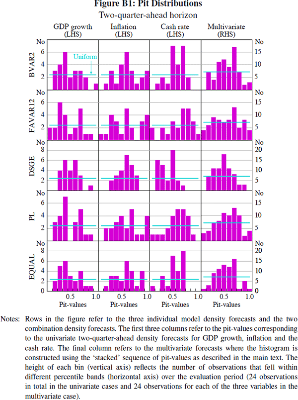
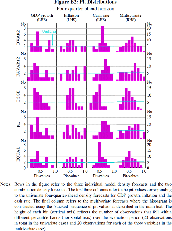
Figures B1 and B2 present a visual assessment of the hypothesis that the pit-values corresponding to the two- and four-quarter-ahead density forecasts are uniformly distributed.


Table B1 reports p-values for likelihood ratio tests of the null hypothesis that the density forecasts are correctly specified at different forecast horizons. The test is a variant of the tests suggested by Berkowitz (2001) and is described in Elder et al (2005) with two degrees of freedom. The results are broadly in line with the visual assessment of the uniformity hypothesis conducted in the main text, although it is difficult to make a direct comparison. According to the tests, the univariate density forecasts of GDP growth and the cash rate were, in general, poorly characterised, while the inflation density forecasts tended to fare better. We were unable to reject the null hypothesis at the 95 per cent significance level that the BVAR12, FAVAR12, and predictive-likelihood weighted combination density forecasts for inflation were not misspecified at any forecast horizon. The test of correctly-specified multivariate density forecasts proved difficult to pass, and except for the FAVAR12 model at the one- and two-quarter-ahead forecast horizons, the null hypothesis that the multivariate density forecasts coincide with the actual joint density was rejected at the 95 per cent significance level. Again, there is little evidence to suggest that the ‘optimally’ combined density forecasts are superior to the best-performing individual model or the equally weighted forecasts, although the small sample makes it difficult to draw strong conclusions.
| GDP growth | Inflation | Cash rate | Multivariate | |
|---|---|---|---|---|
| One-quarter-ahead horizon | ||||
| BVAR2 | 0.00 | 0.09 | 0.00 | 0.00 |
| FAVAR12 | 0.01 | 0.90 | 0.24 | 0.24 |
| DSGE | 0.00 | 0.00 | 0.01 | 0.00 |
| PL | 0.01 | 0.25 | 0.00 | 0.00 |
| EQUAL | 0.00 | 0.01 | 0.00 | 0.00 |
| Two-quarter-ahead horizon | ||||
| BVAR2 | 0.01 | 0.08 | 0.00 | 0.00 |
| FAVAR12 | 0.02 | 0.78 | 0.18 | 0.30 |
| DSGE | 0.00 | 0.00 | 0.00 | 0.00 |
| PL | 0.01 | 0.23 | 0.00 | 0.00 |
| EQUAL | 0.00 | 0.01 | 0.00 | 0.00 |
| Four-quarter-ahead horizon | ||||
| BVAR2 | 0.01 | 0.11 | 0.00 | 0.00 |
| FAVAR12 | 0.04 | 0.30 | 0.03 | 0.00 |
| DSGE | 0.00 | 0.00 | 0.00 | 0.00 |
| PL | 0.02 | 0.22 | 0.01 | 0.00 |
| EQUAL | 0.00 | 0.01 | 0.00 | 0.00 |
| Eight-quarter-ahead horizon | ||||
| BVAR2 | 0.01 | 0.47 | 0.00 | 0.00 |
| FAVAR12 | 0.01 | 0.59 | 0.00 | 0.05 |
| DSGE | 0.00 | 0.00 | 0.00 | 0.00 |
| PL | 0.01 | 0.64 | 0.00 | 0.02 |
| EQUAL | 0.00 | 0.14 | 0.00 | 0.00 |
| Notes: Numbers in the table are the p-values for the likelihood ratio test of zero mean and unit variance of the inverse normal cumulative distribution function transformed pit-values, with a maintained assumption of normality. Numbers in bold indicate that the null hypothesis is rejected at the 5 per cent significance level. | ||||