RDP 2008-02: Combining Multivariate Density Forecasts Using Predictive Criteria 4. Results
May 2008
4.1 The Sample
The data sample is from 1992:Q1 to 2007:Q3 and as discussed above, a recursive out-of-sample forecasting scheme was used to evaluate each model and generate model weights. The first l = 36 observations (1992:Q1–2000:Q4) were used as the initial training sample to estimate each model before constructing density forecasts up to eight quarters ahead (2001:Q1–2002:Q4). The training sample was then extended by one observation, the models re-estimated and density forecasts over the next eight quarters (2001:Q2–2003:Q1) constructed. Model weights were generated sequentially by repeating this exercise over the remaining sample. The final set of model weights were based on a hold-out sample of 27 observations at the one-step-ahead forecast horizon and 19 observations at the eight-step-ahead horizon (the final training sample was between 1992:Q1 and 2007:Q2, which allows one one-step-ahead forecast to be compared to the final observation). It should be noted that the DSGE model was only re-estimated every four quarters to save on computation time.
4.2 Model Weights
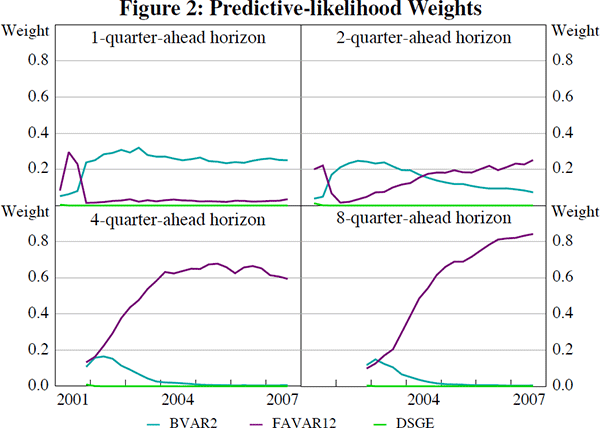
Table 1 shows the final set of model weights (using all observations in the hold-out sample) according to the predictive-likelihood weighting scheme when forecasting one, two, four and eight quarters ahead. Note that a simple unrestricted VAR of GDP growth, trimmed mean inflation and the cash rate (with two to four lags) was also included in the weighting scheme as a benchmark model. How the predictive-likelihood weights evolve throughout the hold-out sample (as the number of observations used to construct the weights increase) is shown in Figure 2 for the BVAR2, FAVAR12 and DSGE models.
| Model | Forecast horizon (h) | |||
|---|---|---|---|---|
| 1 | 2 | 4 | 8 | |
| BVAR4 | 0.22 | 0.32 | 0.00 | 0.00 |
| BVAR3 | 0.18 | 0.11 | 0.00 | 0.00 |
| BVAR2 | 0.25 | 0.07 | 0.01 | 0.00 |
| FAVAR33 | 0.00 | 0.00 | 0.00 | 0.00 |
| FAVAR32 | 0.00 | 0.00 | 0.02 | 0.01 |
| FAVAR23 | 0.00 | 0.00 | 0.00 | 0.00 |
| FAVAR22 | 0.00 | 0.18 | 0.35 | 0.13 |
| FAVAR13 | 0.00 | 0.00 | 0.02 | 0.00 |
| FAVAR12 | 0.03 | 0.25 | 0.59 | 0.84 |
| DSGE | 0.00 | 0.00 | 0.00 | 0.00 |
| VAR4 | 0.02 | 0.04 | 0.00 | 0.00 |
| VAR3 | 0.30 | 0.02 | 0.00 | 0.00 |
| VAR2 | 0.00 | 0.00 | 0.00 | 0.00 |
| Notes: The weights shown in the table are calculated using all observations in the hold-out sample, which is made up of 27 observations for the one-quarter-ahead forecasts and is reduced by 1 observation for each subsequent forecast horizon. | ||||

Table 1 shows that, for forecasting at short horizons, the BVAR model is assigned the most weight. The BVAR specified with 2 lags is preferred at the one-quarter-ahead forecast horizon while 4 lags are preferred at the two-quarter-ahead horizon. The benchmark VAR model specified with 3 lags also receives substantial weight at the one-quarter-ahead forecast horizon. When forecasting at intermediate and longer horizons, the FAVAR model is assigned the majority of the weight. The FAVAR specified with two lags and either one or two factors seems to do the best.
Interestingly, the DSGE model is assigned zero weight at all forecast horizons. This result can be attributed to the large forecast error variance implied by the DSGE model. As we will see in Section 5, the DSGE model's density forecasts were typically too wide (the true degree of uncertainty was over-estimated) when compared with the distribution of actual observations in the sample.
As discussed above, combining weights ‘optimally’ could be troublesome when faced with a small sample of data. Therefore, we also consider an equal-weighting scheme, which assigns a one-third weight (wk,h = 1/3) to the BVAR2, FAVAR12 and DSGE models at all horizons and in all time periods. While an equal-weighting scheme across all 13 models shown in Table 1 could have been used, that approach would tend to overweight the FAVAR models (of which there are 6 different specifications) and underweight the others, in particular the DSGE model.
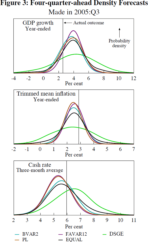
To give a flavour of what the combination density forecasts may look like, Figure 3 shows a cross-section of the four-quarter-ahead density forecasts that would have been made in 2005:Q3 when using the predictive-likelihood and equal-weighting schemes (using weights that would have been available at the time of forecasting). The individual BVAR2, FAVAR12 and DSGE model forecasts are also shown to give an idea of how the combination forecasts differ.

Looking at Figure 3, a couple of points are worth making. The predictive-likelihood combination density forecasts are typically similar to the FAVAR12 model's density forecasts since that model is given a large weight at the four-quarter-ahead forecast horizon. It is also clear that the DSGE model's density forecasts are characterised by a much larger degree of uncertainty than is the case with the other models or the combination density forecasts. Finally, the equally weighted combination density forecast for the cash rate has a ‘fat’ right-hand tail, suggesting that in 2005:Q3, according to this forecast, the risks to the central cash rate projection in four quarters time were somewhat skewed to the upside.