RDP 2008-03: Monetary Transmission and the Yield Curve in a Small Open Economy 5. Unconditional Moments
June 2008
- Download the Paper 319KB
Table 3 compares the theoretical standard deviations of output, inflation, the nominal exchange rate and nominal interest rates, all computed at the posterior mean values of the parameters with their empirical counterparts. The model over-estimates the volatility of output and the short-term interest rate and under-estimates the volatility of inflation, the change in the nominal exchange rate and long-term interest rates. The model's inability to capture the variability of interest rates across the yield curve echoes Shiller's (1979) finding of ‘excess volatility’. While the volatility of the short-term interest rate in the model is 35 per cent larger than that of the data, the volatility of the 10-year interest rate in the data is 3 times that of the model.
|
Model (posterior mean) |
90 per cent confidence interval |
Data (1993:Q1–2007:Q2) |
||
|---|---|---|---|---|
| yt | 0.0178 | [0.0146 | 0.0465] | 0.0066 |
| πt | 0.0020 | [0.0017 | 0.0033] | 0.0055 |
| Δet | 0.0116 | [0.0064 | 0.0182] | 0.0338 |
| R1,t | 0.0023 | [0.0019 | 0.0042] | 0.0017 |
| R8,t | 0.0016 | [0.0014 | 0.0031] | 0.0020 |
| R20,t | 0.0010 | [0.0008 | 0.0019] | 0.0019 |
| R40,t | 0.0006 | [0.0004 | 0.0010] | 0.0018 |
Table 4 compares the actual correlations of foreign interest rates, domestic interest rates, output, the change in the nominal exchange rate and CPI inflation with their theoretical counterparts at the estimated posterior mean parameter values of Tables 1 and 2. The model has mixed success in confronting these dimensions of the data. On the one hand, it fails to capture the pro-cyclical behaviour of the yield curve and the correlations between changes in the nominal exchange rate with output, inflation and the short-term interest rate. On the other hand, the signs of the correlations between interest rates of various maturities and currencies, as well as the signs of the correlations between inflation and interest rates, are correctly predicted by the model.
| Data (1993:Q1–2007:Q2) | |||||||||
|---|---|---|---|---|---|---|---|---|---|
| yt | πt | Δet | R1,t | R20,t | R40,t |  |
 |
 |
|
| yt | 1.00 | ||||||||
| πt | 0.14 | 1.00 | |||||||
| Δet | 0.19 | −0.01 | 1.00 | ||||||
| R1,t | 0.08 | 0.48 | −0.01 | 1.00 | |||||
| R20,t | 0.19 | 0.36 | 0.17 | 0.75 | 1.00 | ||||
| R40,t | 0.16 | 0.34 | 0.18 | 0.69 | 0.99 | 1.00 | |||
 |
0.00 | 0.40 | −0.37 | 0.56 | 0.34 | 0.28 | 1.00 | ||
 |
0.19 | 0.30 | −0.19 | 0.49 | 0.70 | 0.66 | 0.66 | 1.00 | |
 |
0.18 | 0.25 | −0.07 | 0.46 | 0.77 | 0.75 | 0.48 | 0.96 | 1.00 |
| Model (posterior mean) | |||||||||
| yt | πt | Δet | R1,t | R20,t | R40,t |  |
 |
 |
|
| yt | 1.00 | ||||||||
| πt | −0.13 | 1.00 | |||||||
| Δet | −0.01 | 0.66 | 1.00 | ||||||
| R1,t | −0.52 | 0.24 | 0.26 | 1.00 | |||||
| R20,t | −0.65 | 0.32 | 0.06 | 0.93 | 1.00 | ||||
| R40,t | −0.66 | 0.32 | 0.06 | 0.93 | 1.00 | 1.00 | |||
 |
0.07 | 0.19 | 0.08 | 0.65 | 0.57 | 0.56 | 1.00 | ||
 |
0.06 | 0.26 | 0.17 | 0.67 | 0.59 | 0.58 | 0.98 | 1.00 | |
 |
0.06 | 0.26 | 0.17 | 0.67 | 0.59 | 0.58 | 0.97 | 1.00 | 1.00 |
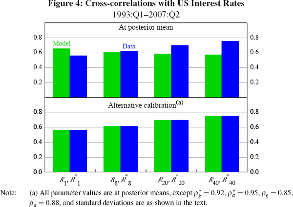
The model's benchmark parameterisation (at the posterior mean) does not generate the upward-sloping pattern of correlations between interest rates of equivalent maturities shown in Figure 1. In particular, the model over-estimates the correlation at the short end of the yield curve and under-estimates it at the long end.
However, there is a set of plausible parameter values capable of producing the upward-sloping
pattern of interest rates correlations in Figure 1. In light of the earlier
discussion about the role that the persistence of shocks plays in accounting
for the moments in Figure 1, we set each of the domestic autoregressive coefficients
to the lower bound of their 90 per cent confidence intervals and the foreign
autoregressive coefficients to their upper
bounds.[15]
Then we adjust the standard deviations of the iid disturbances as follows:
 = 0.0095,
 = 0.013,
  = 0.004,
  = 0.013 and
  =
0.02.[16]
Notice that this alternative calibration changes only the parameters that govern
the exogenous processes, while the deeper model parameters are unchanged.
Figure 4 shows the cross-correlations for the two parameterisations of the
model. The top panel contains the correlations for the parameters at the posterior
mean values of Tables 1 and 2 and the bottom panel contains the correlations
for this alternative parameterisation. For these alternative plausible parameter
values, the model matches the pattern of interest rate correlations at different
points in the yield curve remarkably well.

Table 5 reproduces the contemporaneous correlations in Table 4 for this alternative parameterisation (that is, the one which matches the pattern of interest rate correlations in Figure 1). The most notable differences with respect to the moments computed at the posterior mean are between the correlations of inflation with interest rates and of inflation with output. These parameter values imply that domestic interest rates are somewhat less counter-cyclical, while inflation and output are positively correlated as in the data. However, the correlations between inflation and the yield curve, which are reasonably well-matched to the data in the bottom panel of Table 4, are smaller, though still of the correct sign.
| Model (alternative calibration) | |||||||||
|---|---|---|---|---|---|---|---|---|---|
| yt | πt | Δet | R1,t | R20,t | R40,t |  |
 |
 |
|
| yt | 1.00 | ||||||||
| πt | 0.06 | 1.00 | |||||||
| Δet | −0.03 | 0.59 | 1.00 | ||||||
| R1,t | −0.43 | −0.04 | 0.14 | 1.00 | |||||
| R20,t | −0.41 | 0.19 | 0.04 | 0.92 | 1.00 | ||||
| R40,t | −0.37 | 0.19 | 0.05 | 0.90 | 1.00 | 1.00 | |||
 |
0.15 | 0.11 | 0.04 | 0.56 | 0.68 | 0.73 | 1.00 | ||
 |
0.13 | 0.15 | 0.12 | 0.58 | 0.70 | 0.75 | 0.98 | 1.00 | |
 |
0.13 | 0.15 | 0.12 | 0.58 | 0.69 | 0.75 | 0.98 | 1.00 | 1.00 |
Thus far we have shown that, for plausible parameter values, the model can replicate the correlations between the two yield curves. Hence, in this respect, the theory is consistent with the pattern in Figure 1. However, we can go one step further by analysing not only whether the model can match the data, but whether such a match is likely to occur.[17]
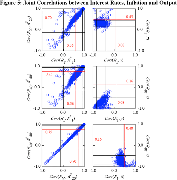
To do this, we take 1,000 draws of the parameters from the posterior density and then calculate the moments of interest for each draw. The blue circles in Figure 5 show the resulting combinations of correlation coefficients for a selection of interest rates, inflation and output. Each plot also shows the 90 per cent confidence intervals computed from these 1,000 draws with dashed lines. The empirical correlations are shown as solid red lines.

Consider the top left panel of Figure 5. This shows the joint posterior distributions of the correlation of the Australian and US 3-month interest rate with the correlation of the Australian and US 5-year interest rate. Both of these empirical correlations lie within the model's 90 per cent confidence intervals. More importantly, the intersection of these empirical correlations lies within the mass of the distribution. This implies that, not only can the model independently match the correlation of Australian and US 3-month and 5-year interest rates, but also that it matches these moments jointly. In other words, the model does not need to sacrifice fit at the short end of the yield curve to match the co-movement at the long end of the yield curve. The results are similar in the remaining two panels on the left side of Figure 5, which show the joint correlations of the 3-month and 10-year, and 5-year and 10-year interest rates.
However, the model is not able to match some of the other correlations. Take, for example, the top-right panel of Figure 5, which shows the joint correlations of the Australian 3-month interest rate with inflation and output. In this case, the empirical correlations lie outside the 90 per cent confidence intervals, suggesting that the model rarely matches these correlations individually. Moreover, the mass of the joint distribution is nowhere near the intersection of the two correlation coefficients. This implies that there is no set of parameter values that allows the model to match jointly these moments of the data. Clearly, the model seems unable to explain the contemporaneous co-movement between output, inflation and interest rates that we observe in the data.[18]
Footnotes
We can gauge the plausibility of these assumptions regarding the relative persistence
of Australian and US shocks as follows. First, noting that our production
function implies that output per capita is a function of labour hours per capita and
productivity, we can back out implied productivity series for Australia
and the US. We can then regress HP-filtered productivity in each country
on a single lag of itself to produce an estimate of the persistence of the
productivity disturbances in each country. The estimated persistence of
the productivity disturbance in the US (equivalent to  in
Equation (6)) was 0.86 and the estimated persistence of the productivity
disturbance in
Australia (equivalent to ρa in Equation (17))
was 0.67.
[15]
The logic behind these changes is as follows. The larger variances of foreign persistent shocks increases the correlations of all rates, but it increases those at the long end of the yield curve relatively more. The larger variance of the domestic monetary policy shock reduces the correlations at the short end, while the larger variances of the persistent domestic shocks reduce the correlations in the middle of the term structure. These values are not unique as it is the relative size of the standard deviations that matter in determining the correlation between foreign and domestic rates. [16]
We cannot determine this with regards to particular parameter values such as those used in the alternative calibration exercise above. To see why, note that while we kept all of the autoregressive coefficients on the disturbance terms within their 90 per cent confidence intervals, it may be that the joint posterior probability of observing that particular combination of parameter values is low. [17]
Elsewhere in the literature, others have found that backward-looking features (such as habit persistence in consumption or indexation in price- or wage-setting behaviour), can help New Keynesian models match some properties of the data. For simplicity, we have used a model that abstracts from these features and left these extensions for further research. [18]