RDP 2013-05: Liquidity Shocks and the US Housing Credit Crisis of 2007–2008 Appendix C: Estimating the Unbiased Aggregate Effect of the Liquidity Shock

Jimenez et al (2011) outline a methodology to estimate the unbiased aggregate effect of the liquidity shock on new lending growth. The model is estimated at the level of the Census tract and the implied coefficient estimates are adjusted for bias using coefficient estimates obtained at the more disaggregated lender-tract level. The approach separates the impact of supply from demand, while taking into account general equilibrium adjustments by borrowers.

It is helpful to outline the methodology in a few steps. For simplicity, suppose there are no control variables. Recall Equation (2) (without controls) estimated at the lender-tract level:

But I want to estimate the tract-level version of this equation:

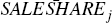
where denotes the log change in credit for tract j across all mortgage lenders. It is a weighted average of the growth rate of credit at the lender-tract level, where the weights are given by each lender's share of loans within each tract. It is not a simple unweighted average of ΔL_j because tracts can start borrowing from new mortgage lenders. The tract-level measure of new lending is constructed by adding up the total number of new loans originated by each mortgage lender within a given tract each year. Similarly, denotes the (weighted) average pre-crisis reliance on loan sales of lenders that grant credit to tract j. This variable is slightly more complicated to construct as it requires converting a measure of the share of loans that are sold by each lender (SALESHARE_i) into a measure of the share of loans that are sold within each tract (). The tract-specific measure of loans sold is constructed using the following formula:

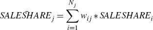
where w_ij = L_ij/L_j is the share of new loans originated by lender i within each tract j and N_j is the set of lenders that originate loans in tract j. Note also that the same credit demand shock (η_j) appears in both Equations (C1) and (C2) under the assumption that the shock affects a tract's borrowing from each lender equally.

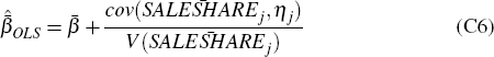
Recall that the OLS estimate of the (partial equilibrium) effect of the liquidity shock at the lender-tract level is given by:

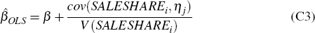
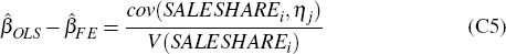
Also, recall that the fixed-effects (FE) estimate (that controls for credit demand shocks) provides an unbiased estimate of the effect of the liquidity shock:

Combining these two conditions we obtain:

Now the OLS estimate of the aggregate (general equilibrium) effect of the liquidity shock at the tract level is given by:

But this will be biased if there is any correlation between the share of loans sold in a particular tract and unobservable tract-specific trends, such as shocks to local housing prices. We cannot follow the same procedure as before and estimate a fixed-effects version of Equation (C2) because the unobservable tract-specific fixed effect (η_j) is collinear with the key explanatory variable (). However, if the correlation between the share of loans sold and the demand shocks is the same across all banks, then the following condition holds:

Combining Equations (C5), (C6), (C7) we obtain the aggregate bias-adjustment formula:

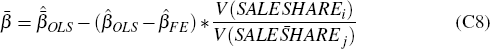
This is the formula used to obtain the unbiased estimate of the aggregate effect of the liquidity shock presented in the paper. Importantly, both the variance of the bank-specific liquidity shocks (V(SALESHARE_i)) and the variance of the (weighted) tract-specific liquidity shocks (V()) can be obtained from the data. This means that all the terms on the right-hand side of the equation can be estimated, providing an unbiased estimate of the aggregate effect of the liquidity shock .