RDP 2013-10: Stochastic Terms of Trade Volatility in Small Open Economies 4. The Impact of Volatility Shocks: Empirics

4.1 Vector Autoregression

To investigate the broader macroeconomic consequences of terms of trade volatility, this section models the responses of real GDP (y), consumption (c), investment (i), the current account (ca) and the GDP deflator (p) to the terms of trade volatility shocks identified in the previous section. Because the economies in our sample have each experienced relatively few sizeable volatility shocks we pool the data for all six countries and estimate a VAR of the form:

where = (y,c, i,ca, p) is a vector of stationary endogenous variables, ν is a vector of constants, = (q_it, σ_q,it) is a vector containing the level of the terms of trade as well as its volatility, is an error vector, A(L) and B(L) are matrix polynomials in the lag operator and var(u_it) = Ω.^[7] Note that although the variables in Y_it respond to the level of the terms of trade and its volatility, neither of the terms of trade variables appear as endogenous variables in the VAR. This is consistent with our assumption in Section 3 that small open economies' terms of trade are exogenous with respect to domestic economic developments.

The empirical model described in Equation (3) can be thought of as a simplified reduced form version of a DSGE model with stochastic volatility, like the one described in Section 5 below. Of course, the empirical model cannot fully capture the non-linear relationships implied by a theoretical model. However, we argue that it nonetheless provides a meaningful indication of the relationships between terms of trade volatility shocks and macroeconomic outcomes that exist in the data, and serves as a useful benchmark against which to compare the results of our theoretical model. In Appendix E we provide additional evidence to support this contention.

4.2 Results

To illustrate the consequences of a terms of trade volatility shock, we report the dynamic effects of an innovation to σ_q of 0.22, roughly equivalent to the average of η_q across the countries estimated in Section 3. After the initial shock, we allow σ_q to decay by 10 per cent per quarter, again broadly consistent with the estimates in Section 3.

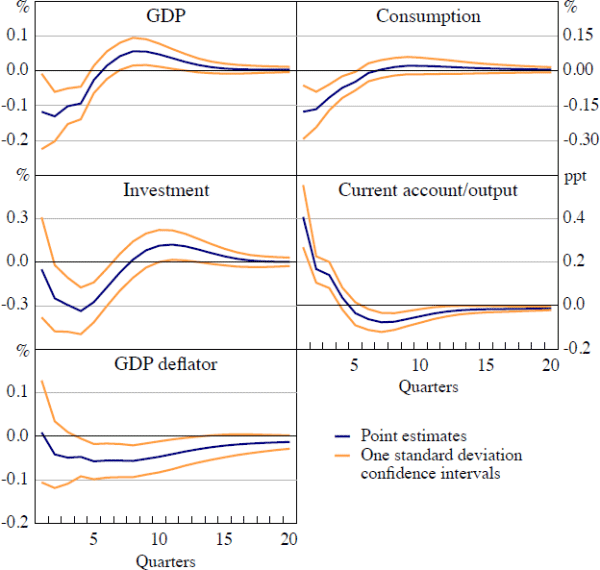
Figure 3 shows the dynamic response of y_it, c_it, i_it, ca_it and p_it to an increase in the volatility of terms of trade shocks, holding the level of the terms of trade fixed. Dark lines indicate the point estimates of the impulse response functions and the lighter lines represent one standard deviation (16th and 84th percentile) of the distribution of responses.

The volatility shock reduces both consumption and investment on impact. Although the investment response is not initially significant, it becomes so in later quarters, and is largest two quarters after the shock. Consumption and investment both return to their original levels eight quarters after the shock, and there is some evidence of a pick-up in domestic demand in later quarters. Aggregate output also decreases in the periods after the shock. The size of its response is smaller than the responses of consumption and investment, however, suggesting an offsetting response of net exports. This shows up in the current account balance (expressed as a ratio to GDP), which increases in the quarter in which the shock hits. It remains above its trend level for two subsequent quarters, before declining as domestic demand recovers. There is also a persistent decrease in the GDP deflator. As we have held the terms of trade constant in this exercise, absent nominal exchange rate movements this implies a fall in the price of non-tradeable goods relative to tradeables.

In reality, of course, both the level of the terms of trade and its volatility may change at any point in time. Empirical studies usually conclude that an increase in the terms of trade has an expansionary effect while a contraction in the terms of trade contracts activity (Broda 2004). Our results suggest that a terms of trade boom that is accompanied by an increase in volatility will have a less expansionary effect than would be the case if terms of trade volatility were to remain constant. In contrast, a fall in the terms of trade will have a larger contractionary effect on activity if it is accompanied by an increase in volatility. In sum, increased terms of trade volatility dampens the effect of terms of trade booms but exacerbates the effect of terms of trade declines.

A possible criticism of our empirical approach is that pooling data conceals cross-country heterogeneity in the impact of volatility shocks. In particular, one might expect that economies in which households and firms are less able to hedge the risks associated with terms of trade volatility will be more responsive to these types of shocks. As a first step to answering this question, Figures 4 and 5 show responses to volatility shocks when we separate our sample into emerging economies – Brazil, Mexico and South Africa – and advanced economies – Australia, Canada and New Zealand.

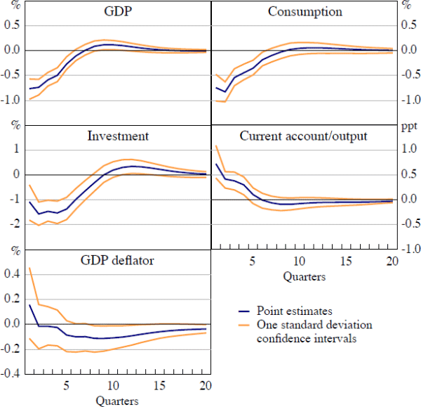
As Figure 4 shows, the effect of volatility shocks on output and its components appears to be larger when we estimate the model on a sample including only the emerging economies. The responses of these variables is roughly four times as large and the changes in investment and GDP are now significant from the quarter of impact. It also takes an additional quarter or two for these variables to return to trend after the shock. The current account-to-GDP ratio continues to increase following the shock, consistent with the contraction in domestic demand exceeding the decrease in GDP. The point estimate of the response of the GDP deflator is qualitatively similar to the pooled response, although it is only marginally statistically significant.

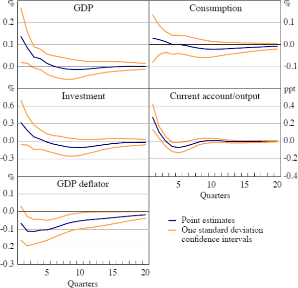
Figure 5 reveals a somewhat different response to the shock among the advanced economies. The responses of investment and consumption for these economies are not significantly different from zero. The initial response of aggregate output is also positive, albeit only significant in the period in which the shock hits. In contrast, the response of the GDP deflator remains negative and significant, and is larger relative to the response of the other variables than in Figure 4. These economies also experience a substantial increase in their current account following the volatility shock.

In sum, the empirical results suggest that, holding steady the level of the terms of trade, an increase in terms of trade volatility triggers a decrease in domestic demand that is partly offset by an increase in net exports, leading to a relatively small impact on aggregate output. These shocks also cause a decrease in the domestic price level which, given that we have held the level of the terms of trade constant, suggests a relative decrease in the price of domestic non-tradeable goods. There is some evidence that the response of output and its components is larger in emerging economies, while the price response is larger in advanced economies. However, given the relatively small number of countries in our sample, we are reluctant to place too much weight on this conclusion. In the following section, we show that a standard international real business cycle model, augmented with stochastic terms of trade volatility, is broadly able to replicate these responses. We then use the model to shed light on the sectoral implications and theoretical causes of these responses.

Footnote

In the results below, we include four lags of the endogenous variables and the contemporaneous value and one lag of the terms of trade variables. Experiments with alternative lag structures produced broadly similar results. We apply an HP filter to the macroeconomic variables to ensure stationarity. [7]