RDP 2013-10: Stochastic Terms of Trade Volatility in Small Open Economies 6. Results
August 2013 – ISSN 1320-7229 (Print), ISSN 1448-5109 (Online)
- Download the Paper 1.06MB
In this section, we analyse the quantitative implications of our model. First, we demonstrate that the model can successfully match some broad features of the macroeconomic data. Second, we show how an increase in terms of trade volatility affects the other variables in the model. Third, we quantify the contribution of terms of trade volatility shocks to the variance of the key macroeconomic variables in the model.
6.1 Moments
Table 6 compares the moments of the model to those of the data. The model matches the three calibrated moments – the variance of output, the relative variance of investment and the level of net exports relative to output – successfully for all countries. The model also comes reasonably close to matching the correlation of output with consumption. However, it is less successful at replicating some of the other moments of the data. In particular, the volatility of consumption relative to output is generally lower in the model than it is in the data. This is a common finding in small open economy real business cycle models and is generally resolved by assuming the absence of wealth effects on labour supply or adding trend growth shocks to the model (Correia, Neves and Rebelo 1995; Aguiar and Gopinath 2007).[12] The model also produces too much correlation between net exports and income and too little correlation between investment and income. The latter result might be due, in part, to our assumption that all investment goods are imported. We examine this issue in the robustness checks section below.
| Australia | Brazil | Canada | ||||||
|---|---|---|---|---|---|---|---|---|
| Data | Model | Data | Model | Data | Model | |||
| σy | 1.35 | 1.36 | 1.52 | 1.52 | 1.38 | 1.38 | ||
| σc/σy | 0.81 | 0.52 | 1.06 | 0.47 | 0.83 | 0.46 | ||
| σi/σy | 2.97 | 2.96 | 3.67 | 3.67 | 2.97 | 2.97 | ||
| ρc,y | 0.49 | 0.49 | 0.62 | 0.80 | 0.80 | 0.81 | ||
| ρi,y | 0.67 | 0.20 | 0.87 | 0.12 | 0.71 | 0.44 | ||
| ρnx,y | −0.22 | 0.61 | −0.26 | 0.55 | 0.18 | 0.57 | ||
| nx/y | −0.94 | −0.94 | 0.30 | 0.30 | 1.41 | 1.41 | ||
| Mexico | New Zealand | South Africa | ||||||
| Data | Model | Data | Model | Data | Model | |||
| σy | 2.43 | 2.43 | 1.39 | 1.39 | 1.60 | 1.60 | ||
| σc/σy | 1.16 | 0.50 | 1.04 | 0.54 | 1.29 | 0.69 | ||
| σi/σy | 1.82 | 1.82 | 4.46 | 4.46 | 3.70 | 3.70 | ||
| ρc,y | 0.97 | 0.66 | 0.76 | 0.43 | 0.76 | 0.00 | ||
| ρi,y | 0.83 | 0.20 | 0.83 | 0.26 | 0.64 | 0.37 | ||
| ρnx,y | −0.07 | 0.63 | −0.18 | 0.58 | −0.52 | 0.64 | ||
| nx/y | −1.53 | −1.53 | 0.80 | 0.80 | 2.53 | 2.53 | ||
| Notes: σj indicates the standard deviation of variable j; ρi,j indicates the correlation between variable i and variable j | ||||||||
6.2 Impulse Response Functions
We now turn to the dynamic response of the economies to a shock to terms of trade volatility. As the pattern of the responses is broadly similar across economies, we focus and describe the Australian case in detail.
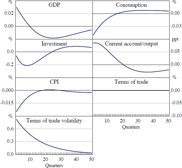
Figure 6 shows the estimated response of the Australian economy to a shock that increases the standard deviation of terms of trade volatility from 2.6 per cent to 6.0 per cent. To put this in context, the shock is of broadly the same magnitude as the estimated increase in Australian terms of trade volatility in the mid 2000s reported in Figure 2.

By construction, the volatility shock has no direct effect on the level of the terms of trade, qt. Despite this, the shock induces a contraction in investment of around 0.2 per cent and in consumption of just under 0.1 per cent. As in the VAR responses, investment displays a ‘hump’ shaped response to the shock. The current account-to-output ratio also increases by around 0.1 per cent following the shock, while the price level decreases. Because the terms of trade does not change following the shock, this implies a decrease in the GDP deflator. The movements in domestic demand and net exports partly offset each other. Consequently, the absolute change in GDP is smaller than the changes in its individual expenditure components. In sum, the model qualitatively matches the empirical responses to a terms of trade volatility shock identified in the VAR, although the the responses are somewhat smaller.
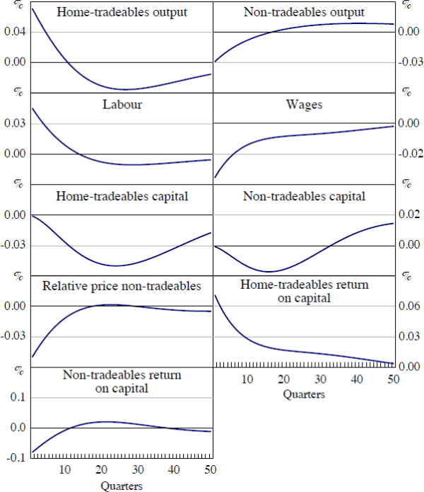
The theoretical model also allows us to trace out the implications of the shock for factor utilisation and the sectoral composition of production (Figure 7). The results suggest that a positive volatility shock leads to an increase in hours worked and a decrease in investment in both the domestic sectors. This change in factor utilisation is associated with a decrease in real wages, while returns to capital in the tradeable goods sector increases. The return to capital in the non-traded goods sector falls, reflecting the contraction in demand for the output of that sector.

Turning to the production side of the economy, the volatility shock brings about a change in the sectoral composition of output away from non-tradeables towards tradeables. The contraction in non-tradeable production follows directly from the decrease in consumption, although this is somewhat mitigated by a fall in the relative price of non-tradeable goods. Domestic consumption of tradeable goods also contracts. However, as wages have decreased relative to the price of tradeable goods, home-tradeable firms find it profitable to expand production. They export this increased production, which contributes to the improvement in the trade and current account balances.
The intuition for the model responses comes from the household's Euler equation:
A shock to terms of trade volatility does not affect the expected level of consumption
directly. But it does make agents more uncertain about their future income.
All other things constant, this increases the expected marginal utility of
future consumption,
 . In response to this, agents reduce
current consumption. This increases the marginal utility of consumption today
and frees up more resources for future consumption, thereby also reducing the
expected marginal utility of consumption in the future. In addition, the reduction
in consumer demand lowers prices today relative to future prices, which decreases
Et {Pt/Pt+1}.
Because the terms of trade is exogenous, the adjustment in prices must occur
through changes in the relative price of non-tradeable goods. Finally, an increase
in volatility also increases the attractiveness of holding foreign assets,
which provide a hedge against a large adverse change in the relative price
of domestic tradeables in the future. In addition to the decrease in consumption,
this explains why the volatility shock is associated with an increase in the
economy's current account balance.
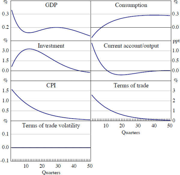
It is instructive to compare the response of the economy to a volatility shock to its response to a shock to the level of the terms of trade, shown in Figure (8). That shock brings about (i) a prolonged increase in consumption; (ii) an investment boom; (iii) an improvement in the current account; (iv) an increase in home-produced goods output and a temporary decrease in non-tradeable goods production; and (v) an increase in hours worked and real wages. These results are consistent with the findings in Mendoza (1995).

Although both shocks lead to an increase in domestic tradeable output and a reduction in foreign debt, the terms of trade level shock is far more favourable to domestic agents. This shock encourages firms to invest in order to increase production to take advantage of temporarily high relative goods prices. The resulting increase in the capital-to-labour ratio drives the increase in real wages, which triggers the expansion in labour supply. However, our results demonstrate that the extent of the expansionary impact of a terms of trade boom will depend upon the degree of terms of trade volatility that an economy experiences. A given increase in the terms of trade will be less expansionary if it occurs during a time of high terms of trade volatility and more expansionary if it occurs when volatility is low.
6.3 Variance Decompositions
In this section we study the contribution to aggregate fluctuations of each of the three shocks in our model. Because we calculate a non-linear approximation to the policy function, it is not possible to assign the total variance to individual shocks as in a linear model. Therefore, in this exercise, we set the realisations of one or two of the shocks to zero and measure the volatility of the economy when we simulate the economy with the remaining shocks.
We study four macro-aggregates: output, consumption, investment and net exports and explore four scenarios: (i) all shocks; (ii) terms of trade level shocks only; (iii) terms of trade level and volatility shocks jointly; and (iv) terms of trade volatility shocks only.[13]
Table 7 reports the variance decompositions for all six countries. For each, productivity shocks are the main contributor for output fluctuations, while shocks to the level and volatility of the terms of trade are key drivers of fluctuations in investment and net exports.[14]
| Australia | ||||
|---|---|---|---|---|
| All | TOT only | TOT + volatility | Volatility only | |
| σy | 1.35 | 0.39 | 0.52 | 0.01 |
| σc | 0.71 | 0.33 | 0.44 | 0.02 |
| σi | 4.03 | 2.83 | 3.77 | 0.06 |
| σnx | 2.56 | 1.84 | 2.43 | 0.03 |
| Brazil | ||||
| All | TOT only | TOT + volatility | Volatility only | |
| σy | 1.52 | 0.37 | 0.51 | 0.06 |
| σc | 0.71 | 0.17 | 0.26 | 0.09 |
| σi | 5.57 | 4.07 | 5.46 | 0.21 |
| σnx | 3.18 | 2.31 | 3.05 | 0.15 |
| Canada | ||||
| All | TOT only | TOT + volatility | Volatility only | |
| σy | 1.38 | 0.21 | 0.26 | 0.00 |
| σc | 0.63 | 0.21 | 0.27 | 0.00 |
| σi | 4.09 | 2.28 | 2.81 | 0.00 |
| σnx | 1.35 | 0.88 | 1.09 | 0.00 |
| Mexico | ||||
| All | TOT only | TOT + volatility | Volatility only | |
| σy | 2.43 | 0.51 | 0.72 | 0.01 |
| σc | 1.21 | 0.44 | 0.62 | 0.02 |
| σi | 4.41 | 2.74 | 3.80 | 0.04 |
| σnx | 3.62 | 2.37 | 3.32 | 0.03 |
| New Zealand | ||||
| All | TOT only | TOT + volatility | Volatility only | |
| σy | 1.39 | 0.46 | 0.56 | 0.01 |
| σc | 0.74 | 0.41 | 0.49 | 0.02 |
| σi | 6.19 | 4.85 | 5.85 | 0.09 |
| σnx | 2.67 | 2.14 | 2.55 | 0.04 |
| South Africa | ||||
| All | TOT only | TOT + volatility | Volatility only | |
| σy | 1.60 | 0.76 | 0.87 | 0.00 |
| σc | 1.10 | 0.82 | 0.94 | 0.00 |
| σi | 5.95 | 4.38 | 5.06 | 0.03 |
| σnx | 3.56 | 3.03 | 3.47 | 0.01 |
| Notes: TOT indicates terms of trade; σj indicates the standard deviation of variable j | ||||
By themselves, volatility shocks account for only a very small portion of the standard deviation of output and consumption for all of the countries in our sample. The impact of these shocks for investment and net exports is somewhat greater, although still modest given the high variance of these series.
However, interacted with shocks to the level of the terms of trade, volatility shocks are estimated to have a meaningful impact on macroeconomic outcomes. For example, with only shocks to the level of the terms of trade, the standard deviation of Australian investment is estimated to be 2.83 per cent. With shocks to the volatility as well as the level of the terms of trade, the standard deviation of investment is estimated to be 3.77 per cent, that is, 33 per cent greater.
Indeed, for countries like Australia, Brazil and Mexico, the volatility of the key macroeconomic variables is between 20 and 30 per cent higher when there are both volatility and level shocks than it is when terms of trade level shocks operate alone. That is, for these countries between a fifth and a third of the effect of the terms of trade on macroeconomic volatility comes through changes in the volatility of terms of trade shocks. For countries like Canada, New Zealand and South Africa, the contribution of volatility to the overall effects of terms of trade shocks is smaller. However, even for these countries, our results suggest that between 10 and 20 per cent of the impact of the terms of trade on the key macroeconomic variables is due in part to volatility in the terms of trade.
Because of the non-linear structure of our model, it is difficult to isolate the
exact channels through which interactions between the level and volatility
of the terms of trade affect the macroeconomy. However, much of the explanation
may come from the fact that stochastic volatility increases the variance of
the terms of trade and larger shocks to the terms of trade imply greater macroeconomic
volatility. To see the impact of stochastic volatility on the variance of the
terms of trade, first note that in the absence of stochastic volatility, that
is if
 , then the variance of the terms of
trade, var (qt) is:
In contrast, when stochastic volatility is present, the variance of the terms of trade is:
where χ2 =
 . For Australia, the presence of stochastic
volatility increases the standard deviation of movements in the terms of trade
by almost 50 per cent, from 7 per cent to 10 per cent. Although other effects
are likely to exist, this direct impact appears about large enough to explain
the change in macroeconomic volatility between the scenario with terms of trade
level shocks only and the scenario with both terms of trade level and volatility
shocks.
Footnotes
In our model, one can induce greater consumption volatility by increasing the magnitude of the portfolio adjustment cost, ψ. This makes it more costly for households to borrow and lend, which reduces consumption smoothing. However, we find that an extremely high value of ψ – generally in the order of 0.1 – is required for the volatility of consumption in the model to match that found in the data. And, with ψ at such a high level, the effect of portfolio adjustment costs on the model's dynamics cease to be negligible. [12]
Note that in each decomposition, agents in the model believe that the shocks are distributed according to the law of motion specified in the previous section. Consequently, they will respond to volatility shocks even when the realisation of shocks to the level of the terms of trade is always zero. [13]
This is likely to overstate the importance of productivity shocks, which in our model account for all variation in macroeconomic aggregates not driven by terms of trade shocks. [14]


