RDP 2014-08: The Effect of the Mining Boom on the Australian Economy 3. Modelling the Mining Boom

To gauge the impact of the mining boom requires a comparison to what would have happened otherwise. We use the AUS-M model of the Australian economy to construct a counterfactual simulation of history assuming the boom did not occur. In the following subsections we first explain the model and then the counterfactual.

3.1 The AUS-M Model

The Australian Macroeconomic (AUS-M) model is a large quarterly time series structural model of the Australian economy. It is based on the TRYM model, originally developed by the Australian Treasury. AUS-M builds on TRYM by incorporating input-output based demand systems and more industry and commodity detail. In terms of common labels, AUS-M is a modern Keynes-Klein-style model, to which CGE features have been added.

AUS-M retains many of the overarching features of TRYM, including an intent to fit the data closely and to reflect mainstream thinking in economic policymaking circles. Key macroeconomic properties are similar. Output in both models is essentially demand determined in the short run (with some important exceptions, discussed below), with major components of real GDP(E) estimated by separate time series regressions.

The model has three sectors (the household sector, the business sector and the public sector) and three markets (the product market, the labour market and the financial market). Systems of equations link each sector and each market. Each equation also has a long-run representation, and these are combined to form a steady-state version of the model that is simulated to provide forward values for expectation variables. A more detailed description of the model is in Appendix A.

The macroeconomic responses of the model to the mining boom are largely in line with the academic literature on the Dutch disease, as applied to recent developments by Sheehan and Gregory (2012) and Plumb et al (2013). Our results can be seen as broadly confirming that earlier work. Our main contribution is quantifying the magnitude and timing of the responses and supplying further detail.

Unlike models such as ORANI, GTAP and G-Cubed where parameters are largely imposed, the parameters in AUS-M are mainly estimated on the basis of the historical time series data. Doing so limits the size of the model, so it is not as detailed as a traditional CGE model. The advantage is that the model has a stronger empirical grounding, especially with regard to dynamic adjustments.

The model is updated quarterly and used for detailed forecasting and sensitivity analysis. It is constantly tested against the data, which promotes a close fit to empirical time series relationships. This helps to provide a realistic description of the dynamics in the economy and a coherent explanation of historical developments.

3.2 The Baseline and Counterfactual Simulations

To quantify the effects of the mining boom, we first simulate the model to recreate history up to mid 2013. That involves the construction of time series of residuals for each of the endogenous stochastic variables of the model.

Many of the effects of the mining boom are still unfolding; in particular, many mining projects are transitioning from their construction phase to production. To capture these developments, we extend the baseline to 2030, using the model's standard forecasting routines. Of course, any such extension is debatable and almost immediately out of date. However, our interest is in deviations from the baseline, which are relatively insensitive to the precise level of the baseline.

Extending our baseline to 2030 also facilitates comparisons with other research and models, discussed in Appendix B. Despite the inclusion of future values, we refer to this as the ‘historical baseline’ – an unfortunate but standard terminology.

To construct a counterfactual, we then assume different paths for certain exogenous variables and residuals to construct an alternative ‘history’ in which the mining boom did not occur. Almost all our results compare this counterfactual with our historical baseline. In our view, the mining boom is best viewed as the confluence of several large distinct shocks hitting the Australian economy. This is reflected in the construction of our counterfactual, which proceeds in three major stages, listed below. A few minor adjustments, which are of a more technical nature, are discussed in Appendix C.

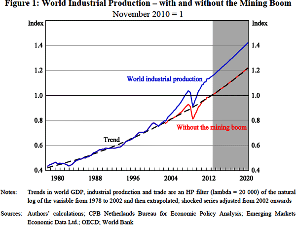
A large part of the run-up in mining prices and investment can be explained as a response to faster economic growth among our trading partners. Accordingly, the first step in constructing our counterfactual is to lower recent world growth and industrial production. We hold the trend growth of world industrial production and other global variables constant after 2002 at their 2002 rates. This results in the level of world industrial production being 13 per cent below baseline by 2013 (Figure 1). In doing so, only the trend growth rate is changed, not the variation around the trend – so for example, the global financial crisis still occurs. The slower growth impacts on agricultural, manufacturing and service exports as well as mining exports.

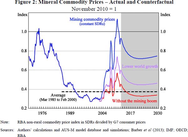
Removing the above-trend growth in global demand is estimated to reduce commodity prices by about 40 per cent, but still leaves them well above previous levels (Figure 2). Implicitly, there appears to have been supply-side as well as demand-side elements to the surge in prices, perhaps reflecting depletion of resources. The second step in constructing our counterfactual is to adjust equation residuals so as to lower world mineral prices (including oil and gas) a further 25 per cent, to bring them into line with average levels from 1985 to 2000.

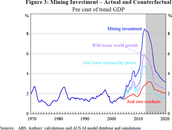
Even with lower world growth and lower minerals prices, investment in Australian mining surges (Figure 3). That is because AUS-M interprets much of the recent strength of mining investment as a response to the discovery of new resources and technology, over and above the usual response to high prices. For example, the development of horizontal drilling and seam fracturing or fracking technology has allowed the exploitation of coal seam and shale gas reserves that previously were difficult if not impossible to tap. At the same time, a combination of factors in Asian energy markets, particularly concerns over energy security, pollution and greenhouse gas emissions, has led to a demand for the sort of long-term contracts that have allowed commitments to be made to build the projects. And some mining discoveries have reflected simple good luck. Some narratives of these developments describe them as a larger-than-normal effect of demand. However, how these unusual effects are labelled is not a substantive issue.

Accordingly, the third major component of our counterfactual is to lower mining investment beyond the response to lower commodity prices, as shown in Figure 3. We implement this by setting residuals in the mining investment equations to zero.

This means that mining investment in the counterfactual can be interpreted as the standard response to economic conditions, without unusual surprises.

Our interpretation of the mining boom reflects one possible set of choices and tools. The experiment could easily be designed in other ways. A simple alternative would be to assume that the changes in prices, investment and output were entirely exogenous. For example, we model the effects of an exogenous change in prices in Appendix B. However, given the predictability of the response of the mining industry to growing world demand, a central scenario that did not model these relationships seemed unrealistic and difficult to interpret.

In the other direction, the boom could be explained at deeper levels, for example by tracing its links back to the growth in Chinese steel demand. In a larger, more complicated model, more dimensions of the mining boom could be explained. However, the level of detail in AUS-M provides a constraint on that. And more fundamentally, our focus is on the consequences of the mining boom, not its causes. In the rest of this paper, we take the above developments as given, and explore their effects.

3.3 Caveats

AUS-M provides a simple description of key economic relationships at a relatively aggregated level, estimated with macroeconomic time series. By design, it ignores differences between detailed industry and commodity classifications. For example, our central experiment concerns a change in ‘mining prices’ and we do not distinguish whether this is a change in iron ore, coal, aluminium or liquefied natural gas (LNG) prices, though in practice these prices have moved differently, with different effects. Nor do we distinguish between where or how the mining is done or by whom. Those differences matter for some purposes, but are beyond the scope of this study. The MMRF model is better suited to address some of these questions. We compare our results with MMRF in Appendix B.

Like all models, AUS-M is a simplification. It relies on data of uneven reliability and applicability. We make many specification choices that others would not necessarily agree with. Human behaviour is not constant and economic structures evolve over time. Economic analysis that involves feedback is complex. Consequently, the model is not meant to be used just in a mechanical way, and results should be interpreted with care.