RDP 2014-09: Predicting Dwelling Prices with Consideration of the Sales Mechanism Appendix B: A Theoretical Example

B.1 Auction Prices

For the auction price mechanism, we use a linear example of an affiliated values auction as discussed by Milgrom and Weber (1982) and Klemperer (1999). We assume each time period (quarter) t that multiple English auctions occur. Each auction (indexed by dwelling a at time t) has n_at risk-neutral bidders (hereafter buyers). Buyers' valuations are given by:

where is buyer i's private signal (estimate) of the worth of dwelling a in quarter t, and ψ_at ≥ 0 is the weight attached to a buyer's own signal and γ_at > 0 is the weight attached to the mean of other buyers' signals.

We assume that each buyers' own estimate of the worth of dwelling a in period t is given by a common component, and an idiosyncratic component :

We assume that is uniformly distributed with support .

We assume buyers participate in an ascending bids English auction – the mechanism commonly used to sell dwellings in Australia – and we abstract from the possibility that sellers can post a reserve price.^[28]

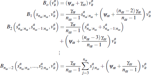
A bidding strategy is given by the prices at which buyers are no longer willing to remain in the auction. The following bidding strategy is consistent with a symmetric equilibrium:

where represents the price at which a buyer with valuation drops out given that k players have previously dropped out of the auction, and is the jth highest signal of the value of dwelling a in period t (and so ). Note that in this equilibrium other buyers' signals can be inferred as they exit the auction. That is, information about the value of the dwelling is revealed through the auction process.

That this is a symmetric equilibrium bidding strategy can be checked by noting that all of the above exit points occur when the buyer with valuation is indifferent to exiting and remaining in the auction, given the observed exit of k players previously.

The equilibrium sale price in this auction is given by the point at which the second-last buyer drops out of the auction, and so there is only one remaining buyer:

Using Equation (B2) we can rewrite Equation (B3) as:

where is the jth highest idiosyncratic component of the estimate of dwelling a's value in period t.

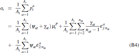
Taking an average price of all auctions that occurred in period (quarter) t, we have:

where A_t is the total number of successful auctions that occurred.

B.2 Private-treaty Prices

We now model price determination in private-treaty negotiations. In particular, we assume that the bilateral negotiation between a buyer and seller is consistent with a Nash bargaining outcome. We assume a single buyer and seller who have valuations for dwelling i in quarter t of:

where idiosyncratic components are drawn randomly from uniform distributions on the intervals and respectively. Again, is the common valuation of the dwelling.

A valid sale requires (we have a valid match) and the match surplus is given by:

With Nash bargaining the negotiated private-treaty sale price is:

where ψ_it ∈ [0,1] is the bargaining weight of the buyer and (1– ψ_it ) is the bargaining weight of the seller.

The average private-treaty sale price given P_t successful private-treaty sales in a quarter will be:

B.3 An Unobserved Components Representation

To link the theoretical models to our empirical findings, we first show that average auction and private-treaty prices admit an unobserved components representation. We then show, given certain restrictions, this unobserved components representation admits a VECM representation with finite lags.

To derive the unobserved components representation of average auction and private-treaty prices, we take asymptotic approximations of each average price. For auctions, we take the approximation as both the number of buyers in each auction and the overall number of auction transactions become large. For private-treaty prices, the approximation is taken as the number of overall private-treaty negotiations (which includes successful and unsuccessful negotiations) becomes large.

B.3.1 Auction prices

Recall that is the jth highest order statistic after n_at random draws from a uniform distribution with support . To conserve notation, we will assume n_at = n for all a and t, without loss of generality. We first discuss convergence of an indiviudal auction price, as n →∞, and then convergence of the average auction price as the number of auctions grows large (approaches infinity).

The equilibrium price for auction a at time t is given by:

Lemma 1. An individual auction converges to a weighted sum of the common component of valuations and the upper bound from which idiosyncratic signals are drawn. That is:

Proof. We begin studying the convergence of the term . First, note that:

And so:

Next note that:

Finally, since ψ_at, γ_at and are not functions of n, we obtain

as required.

Turning to average prices, the average auction price is:

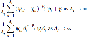
We study convergence of the average price as A_t → ∞; that is, the number of auctions is large. Applying the previous results and assuming that:

it is straightforward to verify:

B.3.2 Private-treaty prices

We next study the convergence of private-treaty prices as the number of bilateral negotiations becomes large. Let be pairs of random draws with each buyer draw from a uniform distribution with support and each seller draw is from a uniform distribution with support , where now refers to the total number of private-treaty negotiations, including those that are successful and those that are not. The average private-treaty price, based on successful transactions, is:

where is an indicator function used to identify successful sales:

We are interested in the convergence of p_t as . That is, as the number of negotiations becomes very large.

Lemma 2. Average private-treaty prices converge to a mixture of common and idiosyncratic components. The idiosyncratic components are a non-linear function of the dispersion of buyers and sellers, and the Nash bargaining parameter. Formally:

where

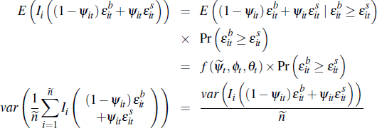
Proof. First notice that:

It is straightforward to show:

This follows since:

where . We have assumed (note ψ_it is statistically independent of the signals and ) and applied Chebyshev's inequality.

Next note:

Bringing these results together and applying Slutsky's theorem:

where the final term is simply given by as required.

B.3.3 Summary of results

In sum, we have established that average auction and private-treaty prices can be approximated in large samples using the unobserved components model:

where is defined in Lemma 2 and we define β_t = ψ_t + γ_t.

Footnote

See Appendix D for the inclusion of seller reserve prices. [28]