RDP 2015-01: Stress Testing the Australian Household Sector Using the HILDA Survey Appendix A: Unemployment Probabilities
March 2015 – ISSN 1448-5109 (Online)
- Download the Paper 1.07MB
We generate an unemployment shock using a Monte Carlo simulation, where each individual's probability of becoming unemployed is estimated using a separate logit model for each year. The probability that individual i is unemployed is:
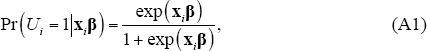
where U is an indicator variable equal to one if individual i is unemployed and equal to zero otherwise, x is a vector of regressors and β is a vector of coefficients. To select the regressors, we use a general-to-specific modelling approach for 2010, removing insignificant variables to arrive at a parsimonious model (Table A1).[17] All remaining variables are significant, or for categorical variables jointly significant, at the 5 per cent level. The same regression is replicated for 2002 and 2006.
The signs of each marginal effect are generally as expected, although there is some variability across surveys. Previous spells of unemployment, less education, not being born in an English-speaking country, not being married, being a single parent, being Aboriginal or Torres Strait Islander, not earning rental income or being in poor health increase the probability of being unemployed. Up to a point, ageing makes individuals less likely to be unemployed.
Examining the size of each marginal effect gives us an idea of which variables have the greatest effect on our predictor of unemployment. Using a base case, where all categorical and dummy variables are set to the sample mode and continuous variables to the sample mean, demonstrates that many variables in our regression have sizeable effects on unemployment; for example, relative to the base case, being unemployed for at least one year prior to the survey increases the base case individual's probability of being unemployed by between 16 and 40 percentage points in each year. Conversely, a university education reduces the probability of being unemployed by 3–5 percentage points.
| Variable | Marginal effects (ppt) | ||
|---|---|---|---|
| 2002 | 2006 | 2010 | |
| Aboriginal or Torres Strait Islander | 9.7 | 11.8*** | 27.9*** |
| Age (quadratic term included) | −0.2*** | −0.2*** | −0.3*** |
| Born in English-speaking country | −4.1*** | −2.4*** | −3.6*** |
| Earns rental income | −4.8*** | −1.8 | −2.9** |
| Educational attainment | |||
| Completed year 12 | −4.2*** | −2.5*** | −4.0*** |
| Diploma | −3.4*** | −2.0*** | −3.8*** |
| University | −5.2*** | −3.2*** | −4.5*** |
| Family structure | |||
| Couple with dependent children | −1.9 | −0.1 | 1.3 |
| Couple without dependent children | −2.8 | 0.1 | −0.1 |
| Single with dependent children | 7.5*** | 5.7*** | 5.7*** |
| Long-term health condition | 10.7*** | 7.2*** | 5.8*** |
| Married | −1.0 | −1.4 | −2.9** |
| Previously unemployed for at least one year | 39.5*** | 16.2*** | 21.1*** |
| Pseudo-R2 | 0.19 | 0.17 | 0.17 |
| Number of observations | 8,604 | 8,789 | 9,179 |
|
Notes: Base case sets categorical variables to their mode and continuous variables to their mean; *, **, *** denote significance at the 10, 5 and 1 per cent levels, respectively, for the test of the underlying coefficient being zero; marginal effects calculated for categorical variables as a discrete change from the base case and for continuous variables as a one-unit change Sources: Authors' calculations; HILDA Release 12.0 |
|||
Footnote
The variables in the initial regression were similar to those in Buddelmeyer, Lee and Wooden (2009). [17]