RDP 2015-01: Stress Testing the Australian Household Sector Using the HILDA Survey 5. Results
March 2015 – ISSN 1448-5109 (Online)
- Download the Paper 1.07MB
5.1 Pre-stress Results
Prior to applying shocks, we review the pre-stress results to: (1) quantify household financial resilience; (2) estimate the financial system's exposure to households with negative financial margins; and (3) assess changes in these measures through the 2000s. This exercise also allows us to compare our results against those of other studies.
5.1.1 Financial margins
According to the model, the share of households with negative financial margins was 12 per cent in 2002, 10 per cent in 2006 and 8 per cent in 2010. These estimates compare reasonably with other literature. For example, using the ABS 2007–08 Survey of Income and Housing and a different definition of basic consumption, Burke, Stone and Ralston (2011) estimate that at least 14 per cent of Australian households had negative financial margins. Albacete and Fessler (2010), whose approach is comparable to our own, estimate that 5.6–9.2 per cent of Austrian households had negative financial margins.[8]
Renters were more likely to have negative financial margins than owner-occupiers, and lower-income households were more likely to have negative financial margins than higher-income households (Figure 3). Renters and lower-income households were also the main source of the decline in the share of households with negative financial margins over the decade. In contrast, the share of higher-income households with negative financial margins rose slightly in each year. Households with younger heads were more likely to have negative financial margins than households with older heads; this is broadly consistent with consumption-smoothing theories, where younger households borrow against future income to maintain relatively smooth consumption over their life cycle.
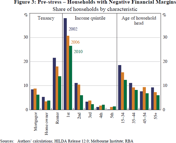
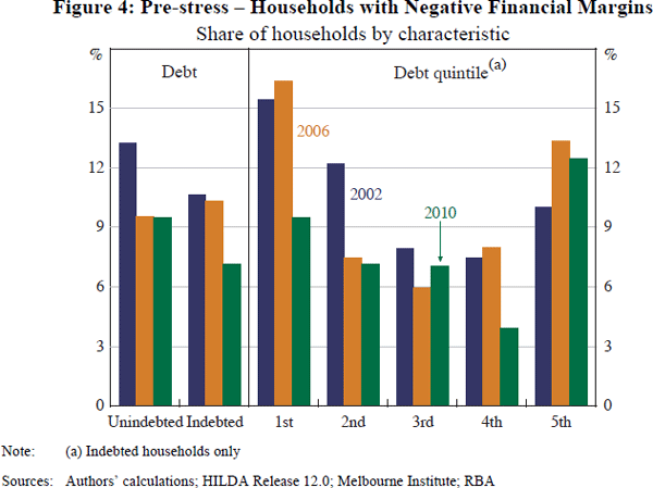
Interestingly, indebted households were not necessarily more likely to have negative financial margins than unindebted households (Figure 4). In addition, the share of households with a negative financial margin tends to decrease as debt increases, although it increases for the highest debt quintile. These findings are consistent with Worthington (2006), who finds that indebtedness is only weakly correlated with financial stress. Furthermore, this result could be interpreted as evidence that the screening lenders carry out in assessing loan applications is broadly effective. That is, before granting a loan, lenders are able to effectively predict whether potential borrowers will be able to comfortably service the loan given their income and other expenses.
It is important to note that most of the households with negative financial margins in the model will not actually default in reality.[9] One reason for this is that households often have assets that they can draw on, so they may actually be in a sound financial position despite having a negative financial margin. We estimate that, in all three years, at least one-third of households with negative financial margins had enough liquid assets – defined here as deposits, equities and trusts – to avoid default for at least one year. If households were able to sell less-liquid assets (such as property), then over three-quarters of households with negative financial margins may have been able to avoid default for over one year.
5.1.2 Debt at risk
As discussed above, LGD (and thus DAR) depends on the collateral that is assumed to be recoverable by the lender in the event of default; assuming that this collateral consists of housing assets only, pre-stress DAR was 0.8 per cent in 2002, 1.2 per cent in 2006 and 1.5 per cent in 2010.[10] The increase in DAR means that even though the share of households with negative financial margins fell over the period, on average these households owed a larger share of debt and/or held less valuable collateral relative to their debt. Overall, however, lenders' exposure to households with negative financial margins appeared fairly limited throughout the 2000s.
By product type, the rise in DAR was mostly driven by credit card and other personal lending (which are generally unsecured). Indeed, the LGD on credit cards and other personal loans averaged around 50 per cent and 25 per cent in each year, respectively (although these loan types only account for about 10 per cent of household debt). DAR on primary mortgages and other property loans remained close to zero in all years, predominantly because Australian housing loans tend to be well-collateralised; each year, less than 5 per cent of owner-occupier mortgagors said that the value of their home was less than their outstanding mortgage. In contrast, DAR on other housing loans, such as second mortgages and investor housing loans, was around 1 per cent. To some extent, the assumption in the model that households default on other debt before housing loans drives these results by driving down LGDs on housing loans and pushing up LGDs on other loans.
The rise in DAR over time is also broadly consistent with actual outcomes; the impairment rate on banks' household loans rose through most of the 2000s and peaked at about 0.2 per cent in June 2011. Moreover, the relative levels of DAR by product type in 2010 compare reasonably with the relative levels of actual portfolio losses experienced by three of Australia's four largest banks over the same period; annualised net write-offs reported by the three banks averaged 3 per cent between 2010 and 2012 for both credit card and other personal lending, while the write-off rate on housing lending was much lower, at 0.04 per cent.[11]
5.2 Macroeconomic Shocks
The effects of shocks to interest rates, the unemployment rate and asset prices are assessed individually. Applying each macroeconomic shock in isolation gives a sense of its effect on household credit risk in the model, even though the shocks would not typically occur in this manner in a real-world scenario. Additionally, this section explains how each of these shocks operates in the model.
5.2.1 Interest rates
An increase in interest rates leads to an increase in debt-servicing costs for indebted households, lowering their financial margins. Therefore, interest rate rises tend to increase the share of households with negative financial margins, and thus the share of households assumed to default. Interest rate shocks are assumed to pass through in equal measure to all household loans.[12]
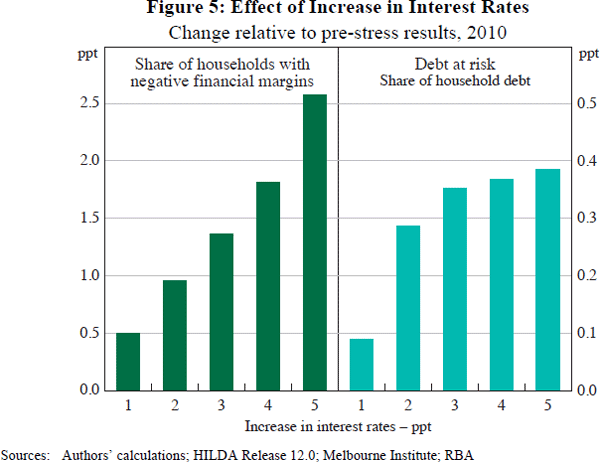
A 1 percentage point rise in interest rates causes the share of households with negative financial margins to increase by 0.5 percentage points and DAR to rise by 0.1 percentage points (Figure 5). The impact on DAR is limited because the households whose financial margins are reduced below zero by the rise in interest rates tend to have debt that is well collateralised. Indeed, on average, the households whose financial margins fall below zero due to the shock have debt that is better collateralised than that of the households that already had negative financial margins (i.e. LGD falls after the interest rate shock). For larger increases in interest rates, the share of households with negative financial margins increases approximately linearly. In contrast, the effect of interest rate increases on DAR is nonlinear.
5.2.2 Unemployment rate
A rise in the unemployment rate causes the income of those individuals becoming unemployed to fall to an estimate of the unemployment benefits that they would qualify for, lowering the financial margins of the affected households.[13]
Methods for simulating unemployment rate shocks differ throughout the literature. Albacete and Fessler (2010) set whole households to enter unemployment, where the probability that each household becomes unemployed is estimated using a logit model. Fuenzalida and Ruiz-Tagle (2009) allow individuals to become unemployed, with unemployment probabilities estimated using survival analysis. Holló and Papp (2007) and Sveriges Riksbank (2009) assume that each individual has an equal probability of becoming unemployed.
Our approach uses a logit model to estimate the probability of individuals becoming unemployed. This means that unemployment shocks in the model will tend to affect individuals with characteristics that have historically been associated with a greater likelihood of being unemployed. The unemployment probabilities are perturbed to yield unemployment rate shocks. Post-stress results are presented as the average of 1,000 Monte Carlo simulations using these probabilities. For details on how the unemployment probabilities are generated, see Appendix A.
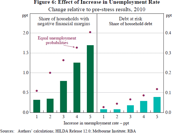
A 1 percentage point increase in the unemployment rate raises the share of households with negative financial margins by 0.3 percentage points (Figure 6). A 5 percentage point rise in the unemployment rate causes this share to rise by 1.7 percentage points. Despite the rise in the share of households with negative financial margins, the unemployment rate shock has little impact on DAR in each year. This result largely reflects the limited debt and good collateral position of the households most likely to become unemployed. Assigning equal probabilities of unemployment to all individuals increases the effect of the unemployment rate shock on both the share of households with negative financial margins and DAR.
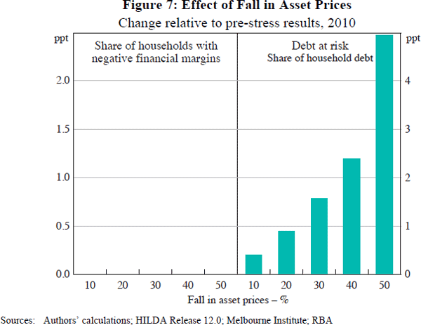
5.2.3 Asset prices
Falling asset prices increase LGD but have no effect on the share of households with negative financial margins. We assume that a given asset price shock applies equally to all households.
A 10 per cent fall in all asset prices causes DAR to rise by 0.4 percentage points (Figure 7). A 50 per cent fall in all asset prices causes DAR to rise by 5 percentage points. Mortgagors are the most affected by this shock, particularly younger mortgagors, because they tend to have paid down relatively little of their loans and have experienced limited cumulative growth in dwelling prices.
5.3 Stress-testing Scenarios
The following simulations apply the above shocks in combination to examine household resilience under two scenarios, labelled ‘historical’ and ‘hypothetical’ (as described below). The magnitudes of the shocks under each of these scenarios are shown in Table 3, while Figure 8 overlays the shocks against aggregate data.
| Historical | Hypothetical | |
|---|---|---|
| Change in assets prices (per cent): | ||
| Housing | −5 | −25 |
| Equities | −50 | −25 |
| Retirees' superannuation and trust funds | −30 | −25 |
| Other(a) | 0 | −25 |
| Change in unemployment rate (ppt) | 2 | 6 |
| Change in cash rate (ppt) | −3 | 0 |
| Note: (a) Includes collectible and vehicle assets | ||
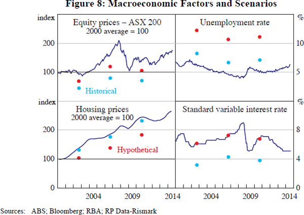
The ‘historical’ scenario is designed to roughly replicate the change in macroeconomic conditions that occurred in Australia during the global financial crisis. This includes a sharp fall in equity prices, a moderate fall in housing prices, a slight rise in the unemployment rate and an offsetting large fall in interest rates.
The ‘hypothetical’ scenario is calibrated similarly to the stress-test scenario in APRA (2010), in which a global deterioration in economic conditions causes a downturn in Australia that is significantly worse than that experienced in the early 1990s. Compared to the historical scenario, the fall in equity prices is smaller, the decline in housing prices and the rise in the unemployment rate are larger, and there is no offsetting change in interest rates.
The results from the scenarios should be interpreted as indicating the effects of stress on household financial resilience and how these effects have changed over the 2000s. However, it is important to keep in mind the assumptions underlying the model, and its limitations. Some of these limitations are outlined in Section 6.
5.3.1 Historical scenario
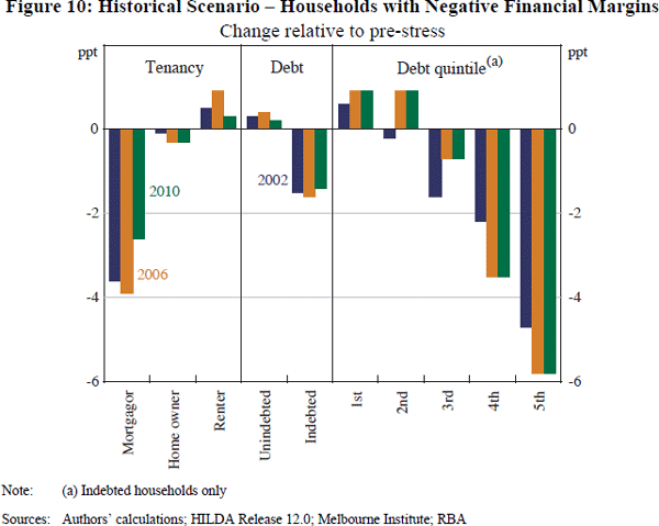
Under the historical scenario, the share of households with negative financial margins falls in all years by around 1 percentage point relative to the pre-stress baseline (Figure 9). This is due to the fall in interest rates, which more than offsets the rise in unemployment. This result illustrates the potential for expansionary monetary policy to offset the effects of increases in unemployment on household loan losses; by reducing debt-servicing costs, the interest rate reduction increases financial margins and thus makes borrowers less likely to default.[14] The decline in the share of households with negative financial margins is largest for the most indebted households, which are typically mortgagors (Figure 10). The share of households with negative financial margins rises for renters and those with little or no debt. Relative to the pre-stress scenario, LGD rises in each year due to the fall in asset prices. However, the decrease in the share of households with negative financial margins means that DAR declines (Figure 9).
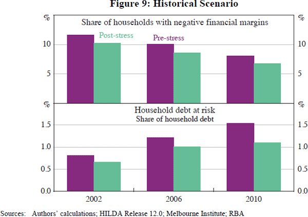
As noted, the results from the historical scenario are driven by the strong offsetting effects of lower interest rates in the model. While this may partially reflect the simple nature of the model, Australia's experience during the global financial crisis suggests that it is not implausible; with the assistance of accommodative monetary policy, the Australian economy was able to absorb a shock of similar magnitude during the crisis with limited aggregate impact on household loan performance.
5.3.2 Hypothetical scenario
The hypothetical scenario is much more severe, along most dimensions, than the historical scenario. Accordingly, under this scenario, the share of households with negative financial margins increases by around 2 percentage points in each year, to a total of 13 per cent in 2002, 11 per cent in 2006 and 10 per cent in 2010 (Figure 11).
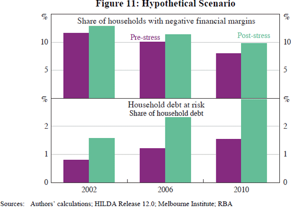
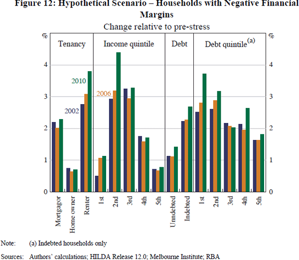
Under this scenario, households in the middle of the income distribution and renters are the most affected (Figure 12). Households with younger heads are also affected, while household with older heads are not especially affected in any year, suggesting that the increase in indebtedness among these households through the 2000s did not significantly expose the household sector to additional risks. Households with debt are more likely to be impacted by the scenario than those without debt. However, of those households with debt, the impact of the scenario is greatest on those with relatively little debt.
Under the hypothetical scenario, post-stress DAR increases relative to pre-stress DAR in each year (Figure 11). This result is largely because of the fall in asset prices, which causes the LGD to rise (but has no effect on the frequency of default). The magnitude of the difference between pre- and post-stress DAR (i.e. the effect of the shock on DAR) increases over time, to peak at about 1.5 percentage points in 2010.
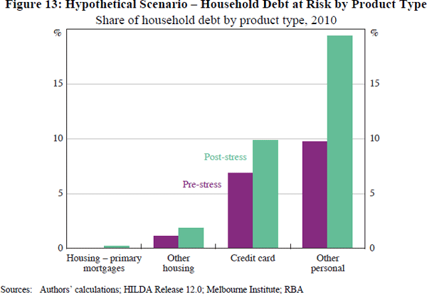
The increase in expected losses on credit card and other personal debt drives the rise in household DAR; DAR on other personal loans doubles to nearly 20 per cent (Figure 13). By comparison, the rise in DAR on primary housing loans is small, largely because of the strong collateralisation of housing loans in Australia (and the assumptions around loss precedence). Regardless, given that housing loans make up the vast bulk of household lending, small changes in DAR on housing loans result in large changes in total household DAR.
The results from the hypothetical scenario suggest that the household sector would have remained fairly resilient to macroeconomic shocks during the 2000s, and that the households that held the bulk of debt tended to be well placed to service it, even during macroeconomic shocks. However, based on this scenario, the effect of macroeconomic shocks on DAR appears to have increased over the 2000s. This suggests that household vulnerability to shocks may have risen a little. This might be because some households were in a less sound financial position following the global financial crisis (for instance, because the labour market had weakened and the prices of some assets had declined). As a consequence, shocks of a magnitude that previously would have left these households with a positive financial margin and/or sufficient collateral so as not to generate loan losses for lenders may, following the crisis, have been large enough to push these households into having a negative financial margin and/or insufficient collateral.
5.3.3 Comparison with bank capital
The stress-testing model in this paper is used to examine household financial resilience over the 2000s. In contrast, stress-testing frameworks that are developed for practical prudential purposes are used to assess the resiliency of the banking sector. Our model design means that we can only make very simple comparisons regarding the size of expected losses under the scenarios relative to bank capital. Nonetheless, this still provides some context for the results by giving a broad indication of the magnitude of the direct flow-on effects to the banking sector from household loan losses (i.e. DAR) generated by the model. Using data from the Australian Prudential Regulation Authority (APRA), we compare the results from the hypothetical scenario to banks' total capital. We assume that pre-stress losses have already been properly provisioned for and that loss rates are equal across lenders (i.e. banks, other authorised deposit-taking institutions (ADIs) and non-ADI lenders, such as mortgage originators).
The DAR results imply that expected losses (under the scenario outlined) on banks' household loans were equivalent to a little less than 10 per cent of total bank capital (on a licensed ADI basis), assuming that eligible collateral consists of housing assets only. As mentioned previously, this result assumes that banks have already provisioned for pre-stress losses, but this may not always be the case, as the deterioration in asset quality may surprise some institutions or may take place before objective evidence of impairment has been obtained. Assuming pre-stress losses are not provisioned for, potential losses as a share of total bank capital roughly double. It is important to reiterate that these estimates are simplistic and could differ to actual losses incurred in reality under this scenario by a large margin. For example, some of these loan losses may be absorbed by lenders mortgage insurance.[15]
Footnotes
Other models that are less comparable to our own also find reasonably similar results. Sveriges Riksbank (2009) estimate 6.3 per cent for Sweden, Herrala and Kauko (2007) estimate 13–19 per cent for Finland, and Andersen el al (2008) estimate 19 per cent for Norway. [8]
As a reference point, personal bankruptcies and other administrations as a share of the adult population averaged only 0.2 per cent per year in the 2000s. [9]
DAR is roughly ½ percentage point lower when collateral is defined more broadly as total household assets less non-retirees' superannuation and life insurance assets (both of which are generally protected from creditors in bankruptcy proceedings). [10]
These data only became available from 2008. One of Australia's largest banks does not publish comparable data. The modelled levels of portfolio losses are not comparable with actual (annual) outcomes because of the instantaneous nature of the model. [11]
All loans are assumed to be variable rate. Data from the Australian Bureau of Statistics indicate that variable-rate loans accounted for about 90 per cent of owner-occupier housing loan approvals on average over the 2000s. [12]
In more complicated models, an unemployment shock could be part of a more general income shock. For example, wages could be made to fall. [13]
This effect relies on reductions in the cash rate being passed on in full and instantaneously to borrowers. Excluding the fall in interest rates, the share of households with negative financial margins increases by around ¾ percentage points relative to the pre-stress baseline in each survey and DAR rises by around 0.2 percentage points. Additionally, the assumption that interest rates on credit cards change one-for-one with the cash rate is unrealistic given the relative stickiness of credit card interest rates. However, even under the assumption that credit card interest rates are unchanged, the share of households with negative financial margins and DAR both fall by a similar amount as under the historical scenario. [14]
Lenders mortgage insurance is often taken out by lenders on loans with loan-to-valuation ratios above 80 per cent, which have made up about one-third of loan approvals in recent years. [15]