RDP 2015-04: The Sticky Information Phillips Curve: Evidence for Australia 2. Model and Estimation

2.1 Sticky Information Phillips Curve

The log of a firm's desired price , relative to the log aggregate price level p_t, is proportional to the output gap:

where x_t is the output gap and α is the degree of real rigidity (the elasticity of a firm's desired relative price with respect to the output gap). The smaller is the parameter α, the greater is the degree of strategic complementarity between firms, reducing the sensitivity of firms' desired price to the output gap.^[2] Each period, a randomly chosen fraction (1−λ) of firms receive updated inflation and output gap forecasts for each quarter in the future.^[3] The remaining λ share of firms do not acquire new information, and continue to set prices based on outdated information. The assumption that a fraction of firms continue to work with outdated information each period enables the SIPC to generate inertial inflation dynamics: only prices set by firms acquiring new information will reflect shocks to inflation and output gap forecasts. Combining Equation (1) with the assumption of a state-independent probability of acquiring new forecasts yields the SIPC:

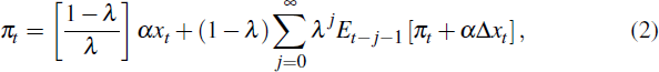
where π_t is the quarterly inflation rate and Δx_t = x_t−x_t−1 is the contemporaneous change in the output gap. Equation (2) indicates that current inflation in part reflects past expectations of current inflation. Mankiw and Reis (2002) motivate the SIPC by relation to a contracting model, in which prices reflect expectations at the time contracts were set. When firms acquire new information, they are assumed to receive rational expectations forecasts. With this assumption, the model resembles Carroll's (2003) epidemic model of information diffusion, in which a random subset of consumers come into contact with professional forecasters each period.

Reflecting the fact that Australia is a small open economy, the baseline closed-economy SIPC is augmented with an import price term, allowing firms' desired price to depend on both the output gap and the cost of imported goods and services. With import prices, Equation (1) generalises to 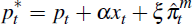, where 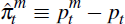is the detrended real log goods and services import price deflator (adjusted for tariff changes). The corresponding open-economy SIPC is given by:

Estimation of the SIPC requires truncating the infinite order lag of expectations and adding an error term ε_t:

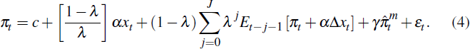
A constant term c has also been added. Because import price forecasts are unavailable, the terms in Equation (3) are omitted; with this simplification, the import price term can be separated from the information rigidity term, noting that γ = (1−λ/λ)ξ.

In general, the output gap term x_t in the SIPC will be correlated with shocks to inflation, in which case ordinary least squares will provide inconsistent estimates of the model parameters. If the error term is iid, any variables known at time t − 1 are valid instruments. But truncating the infinite order lag of expectations is likely to violate this orthogonality condition. The error term ε_t in Equation (4) consists of all forecasts dated t − J − 2 and earlier,

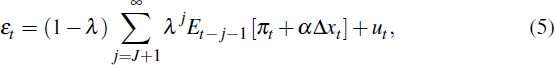
plus an idiosyncratic error term u_t. In general, forecasts dated t − J − 2 and earlier will be correlated with instruments dated t − 1 and earlier. But provided the truncation point is sufficiently long, and λ is not too large, any inconsistency in the parameter estimates is likely to be small. Forecasts dated t − J − 2 and earlier receive weight no greater than (1−λ)λ^J+1, and thus induce a relatively weak correlation between ε_t and candidate instruments dated t − 1 and earlier. Coibion (2010) uses Monte Carlo simulation, and data at a quarterly frequency, to show that for λ = 0.75 (firms update their information set on average once per year), consistent estimation can be achieved with truncation of expectations beyond one year. The set of instruments used to estimate Equation (4) includes the full set of forecasts and the first lag of the output gap. The output gap is the only endogenous variable, and because it is highly correlated with the lagged output gap used as an instrument, the SIPC parameter estimates do not suffer from bias caused by weak instruments.

2.2 New-Keynesian Phillips Curve

For comparison with the SIPC, a NKPC is also estimated. The assumptions underlying the NKPC flip those of the SIPC. The NKPC assumes that firms obtain rational expectations forecasts in each period, but face a restriction on their ability to reset prices: with state-independent probability (1 − θ), a firm is able to reset its price each period. Firms' desired price in each period is given by Equation (1), the same as in the SIPC, but because firms are unable to adjust their price with probability θ in each period, their chosen price when they are free to adjust is a weighted average of their desired price over the expected duration that its price is fixed. This price-setting behaviour implies the following open economy NKPC:

where ρ = ακ, with κ = (1 − θ)²/θ the elasticity of inflation with respect to real marginal cost and, as in the SIPC, α the degree of real rigidity. Often, the driving variable in the NKPC is real marginal cost, rather than the output gap. The output gap is used here for consistency with the SIPC, and because of the relative unreliability of marginal cost estimates.

Import prices are a component of firms' marginal cost, and the sticky-price assumption underlying the NKPC means that changes in import prices are incorporated into consumer prices each period by only a (1 − θ) subset of firms. This implies that the coefficient γ on the import price term is equal to κ multiplied by the share of marginal cost accounted for by import prices: γ = κs. For comparability with the SIPC, this restriction is not imposed.

The NKPC is augmented with an error term and a constant,

The key feature of the NKPC model is the presence of forward-looking inflation expectations, compared to lagged expectations in the SIPC. The NKPC is estimated using the same set of professional and econometric forecasts used to estimate the SIPC. The instrument set consists of the first lag of the output gap, and the time t − 1 forecast of inflation at time t + 1. The most common estimation method for the NKPC replaces expected inflation with its realisation and seeks appropriate instruments. Any pre-determined variable is a valid instrument, but weak identification is a common problem. The use of survey forecasts mitigates this problem: survey forecasts exhibit high serial correlation, in which case E_{t −1} [π_t+1] is a strong instrument for E_t [π_t+1]. But the use of survey forecasts to estimate the NKPC introduces theoretical complications. The NKPC is derived assuming rational expectations, but expectations are non-rational under the SIPC assumptions, because each period firms retain dated forecasts with probability λ. Nonetheless, Mavroeidis, Plagborg-Møller and Stock (2014, p 135) argue that ‘[w]hile the proper microfoundations for price setting under nonrational expectation formation are lacking, the survey forecasts specification may still be taken as a primitive …’. Of particular importance here, the use of forecasts facilitates comparison between the estimated SIPC and NKPC specifications.

Inflation in the NKPC specified by Equation (6) is entirely forward-looking, unlike hybrid specifications that include lagged inflation as an explanatory variable (see, for example, Galí and Gertler (1999) and Galí, Gertler and López-Salido (2005)). The SIPC provides a microfoundation for the inertial behaviour of inflation that the hybrid specification seeks to match in a reduced-form way. The SIPC is compared against a forward-looking rather than hybrid NKPC in order to provide a clear contrast between the alternative sticky-price and sticky-information models of price setting.

Footnotes

This condition can be derived from a firm's profit maximisation condition. See, for example, Blanchard and Kiyotaki (1987). [2]

The SIPC assumes that λ is a structural parameter. See Reis (2006) for a model that microfounds the optimal degree of inattention. [3]