RDP 2015-12: Modelling the Australian Dollar 4. A Markov-switching Model

The rolling ECM described above allows for the possibility that the speed-of-adjustment coefficient evolves smoothly over time. An alternative is to allow for more abrupt changes or ‘switches’ in the model's short-run dynamics. These switches could reflect, for example, sudden but persistent changes in preferences (e.g. during the information technology boom in the early 2000s), risk aversion (e.g. at the onset of the global financial crisis), or other factors which might cause the exchange rate to remain away from its equilibrium for longer than would typically be the case.

If the dates of switches in the model's parameters were known ex ante, standard tests of structural change could be applied to the model. However, as the dates of switches in the model's parameters are unknown, it is necessary to jointly estimate the dates and the magnitude of any change. Markov-switching models are well suited to this task.^[23]

The Markov-switching specification used in this paper allows the ECM's short-run parameters to switch, according to the value of an unobserved binary state variable S_t = {0,1}:

where

for j = 0,…,4.

Since the values of S_t are not known, they need to be estimated. For this purpose it is assumed that S_t follows a first-order Markov-switching process with transition probabilities:

where 0 ≤ p, q ≤ 1.

While all of the model's short-run coefficients are allowed to switch, the underlying Markov states are identified by imposing the restriction γ₀ < γ₁. If there are different states governing the speed of reversion to equilibrium there should be a significant difference between γ₀ and γ₁. Specifically, state S_t = 1 will be associated with a larger (i.e. less negative) speed-of-adjustment coefficient and slower reversion to equilibrium than state S_t = 0.^[24]

As in the case of the rolling ECM, the long-run cointegrating relationship is held constant; with parameter estimates obtained using DOLS.^[25] However, the model's short-run coefficients are estimated over the full sample, so this approach does not suffer from the same loss of information. In line with common recent practice, the ECM is estimated using Bayesian techniques, as outlined in Kim and Nelson (1999). Uninformative priors are adopted to avoid imposing any particular outcome on the model, with the focus on assessing evidence of switching from the data.

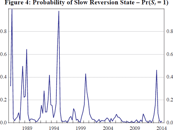
Overall, the model provides limited evidence of switching in the short-run parameters. Over the sample period, there are four quarters where the estimated probability of being in the slow-reversion state (S_t = 1) is above 50 per cent (Figure 4). However, these episodes are short-lived and appear to be fitting outlying observations – where the RTWI has fallen by a large amount and concurrently with the ToT – rather than being indicative of more persistent structural change. Further, the difference between the estimated state-specific speed-of-adjustment coefficients, γ₀ and γ₁, is small, with their posterior distributions overlapping significantly (see Table B1). There are also few meaningful differences in the estimates of most other coefficients in the short-run relationship.

Neither the rolling ECM nor the Markov-switching model find conclusive evidence of unusual influences that have affected the RTWI in recent years (and which are not adequately captured in the existing model). These approaches can be considered ‘agnostic’, in that they allow the data to speak for themselves in identifying changes in the behaviour of the exchange rate, relative to longer-run historical norms.

Another approach, which could be more promising if there are strong ex ante views about what specific additional factors may have exerted a greater influence on the RTWI at different points in time, is to attempt to model these influences directly. Sections 5 and 6 attempt to do this by incorporating a number of additional explanatory variables that may have been revealed as important by two key macroeconomic developments in the past decade, namely: Australia's resources boom (Section 5); and foreign central banks' unconventional monetary policy (Section 6).

Footnotes

Markov-switching models have a wide range of applications in empirical macroeconomics and finance. Applications to exchange rate modelling include: Engel (1994) – who investigated whether Markov-switching models could improve forecasts of exchange rates relative to a random walk with drift, but found little evidence of this – and Hall, Psaradakis and Sola (1997) and Psaradakis, Sola and Spagnolo (2004), who used Markov-switching ECMs to investigate periods of significant deviations of UK housing prices and US equity prices, respectively, from their long-term fundamentals. [23]

The residuals ε_t are assumed to be normally distributed with a mean of zero and constant variance. A version of the model that allowed for switching in the residual variance was also estimated. The results were not materially different from those of the simpler specification and are not reported in this paper. [24]

This approach is similar to Krolzig, Marcellino and Mizon (2002), Hall et al (1997) and Psaradakis et al (2004). [25]