RDP 2015-12: Modelling the Australian Dollar 5. Incorporating Australia's Resources Boom
October 2015 – ISSN 1448-5109 (Online)
- Download the Paper 1.39MB
Over the past decade, Australia has experienced an unprecedented ToT and mining investment boom.[26] Australia's (goods) ToT almost doubled between the end of 2003 and September 2011 (Figure 5). The increase in the ToT has been largely attributed to a significant increase in demand for bulk commodities (such as iron ore) from emerging market economies, which caused prices for these commodities to almost quadruple over the same period (while prices of other, non-bulk, exports rose by around 40 per cent). At the same time, bulk commodities' collective share of Australia's exports rose from around 25 per cent to around 50 per cent.
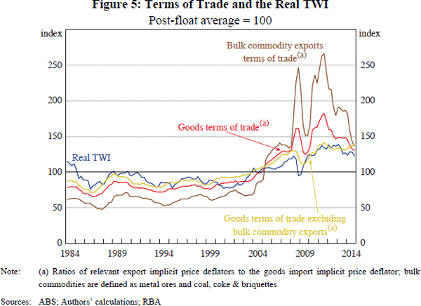
As noted earlier, the ToT has, historically, been a key explanatory variable for Australia's RTWI. Consistent with this, the significant increase in the ToT since the early 2000s also broadly coincided with an appreciation of the RTWI. However, even though changes in the prices of bulk commodity exports have driven most of the variation in the ToT in recent years, the RTWI appears, at first glance, to have had a stronger relationship with a measure of the ToT that excludes bulk commodity export prices. In particular, in recent years, the largest divergences between movements in the RTWI and in the ToT have tended to coincide with particularly large movements in the prices of bulk commodities. This observation raises two key questions:
- Is the relationship between the RTWI and the prices of bulk commodities (as measured in the ToT) different to the relationship between the RTWI and other export prices?; and, if so
- Does the baseline ECM adequately capture the dynamics of the recent ToT boom, insofar as the boom was driven largely by increases in the prices of bulk commodity exports?
In Sections 5.1 and 5.2, we consider two explanations of why bulk commodity export prices could potentially have a different effect on the RTWI than other export prices and augment the baseline model in an effort to capture these differences. In broad terms, the first explanation could be that bulk commodity prices interact differently with the rest of the economy, compared with other export prices (considered in Section 5.1). The second possible explanation is that bulk commodity prices could be less reflective of current expectations than other export prices (considered in Section 5.2).
5.1 The Bulk Commodity Sector's Interaction with the Rest of the Economy
There are at least two key reasons why bulk commodity prices could interact differently with the rest of the economy, compared to other export prices. The first is related to the extent to which the bulks industry is integrated with the rest of the economy (Section 5.1.1) and the second is related to variability in the relationship between bulks prices and investment (Section 5.1.2).
5.1.1 The effect of bulks prices on the rest of the economy
As discussed in Section 3.1, the theoretical literature suggests that variation in the ToT – particularly variation which is driven by changes in global supply of, and demand for, exports – should affect the RTWI. However, the magnitude of this effect is likely to differ depending on which export price(s) caused the variation (Amano and van Norden 1995). This reflects the fact that individual industries could interact differently with the rest of the economy in terms of their use of domestic inputs, their use as an input into other industries' production, their use for domestic consumption and substitutability for other goods, and/or their overall effect on national income.
A number of papers have found empirical support for this notion. For example, both Amano and van Norden (1995) and Maier and DePratto (2008) find that a measure of the ToT which is constructed using only energy export prices has a very different relationship with the Canadian dollar's bilateral exchange rate against the US dollar compared to a measure of the ToT which is constructed using other commodity export prices.
In an Australian context, the export sector that stands out as being potentially unique is the bulk commodities sector. Relative to other export sectors, the bulks sector, and particularly the liquefied natural gas (LNG) sub-sector, uses fewer domestic inputs for production and has a high level of foreign ownership (Connolly and Orsmond 2011; Plumb et al 2013; Rayner and Bishop 2013). Consequently, much of the additional profit associated with higher bulks prices is likely to accrue to foreigners and there will be relatively little additional demand for domestic labour associated with increased production. Overall then, a smaller proportion of the additional income associated with the rise in bulk commodity export prices will actually remain within Australia, suggesting that an increase in the price of bulk commodity exports could have a more limited effect on domestic demand, relative prices and the RTWI than an increase in other export prices (Kent 2014). Similarly, in terms of the nominal exchange rate, there may be only a small increase in net demand for Australian dollars as firms will pay their foreign owners in foreign currency.
If this is the case, the inclusion of bulk commodity export prices in the ToT could make it more difficult to identify a stable relationship between the ToT and the RTWI. While this may have always been an issue, it is likely to have become more prominent in recent years as bulks prices have driven an increasingly large proportion of the variation in the ToT. Decomposing the aggregate ToT into a ‘bulks ToT’ and (an ‘excluding-bulks ToT’ could help to ameliorate this issue and could provide additional insight into the behaviour of the RTWI and its relationship with different export prices.
To examine this, the bulks and excluding-bulks ToT series are included in the ECM's cointegrating relationship separately, in place of the aggregate ToT:[27]
Four different specifications are considered, which vary along two dimensions:
- Weighting scheme: the bulks and excluding-bulks ToT measures are calculated as both ‘unweighted’ and ‘weighted’ measures. The unweighted measures are constructed as the ratios of the bulks and excluding-bulks export price deflators to the total import price deflator. The weighted measures are constructed by multiplying the unweighted bulks and excluding-bulks ToT measures by the (time-varying) bulks and excluding-bulks nominal export shares, respectively. The weighted measures account for the increasing share of bulk commodities in Australia's export basket over the past decade.[28]
- Definition of ‘bulks’: the bulks and excluding-bulks measures are calculated using two definitions of bulk commodities. The ‘narrow’ bulks measure includes only ‘metal ores’, and ‘coal, coke and briquettes’, while the ‘broad’ bulks measure also includes ‘other mineral fuels’ (e.g. LNG).
The results of these models are reported in full in Table 2. Consistent with the observation that the RTWI appears to have been less responsive to movements in bulks prices, the coefficient on the bulks ToT is significantly smaller than the coefficient on the excluding-bulks ToT in all four specifications (weighted/unweighted; broad/narrow) at the 10 per cent level (based on Wald tests). Further, the coefficient on the bulks ToT is only significant at (at least) the 5 per cent level in the two specifications that use the weighted ToT measures.
| Baseline | Narrow | Broad | ||||
|---|---|---|---|---|---|---|
| Unweighted | Weighted | Unweighted | Weighted | |||
| Variables | ||||||
| Constant | 0.41*** (0.11) |
0.32* (0.17) |
0.36* (0.21) |
−0.14 (0.21) |
0.04 (0.24) |
|
| Speed-of-adjustment | −0.22*** (0.05) |
−0.25*** (0.05) |
−0.24*** (0.05) |
−0.23*** (0.05) |
−0.18*** (0.05) |
|
| Equilibrium relationships | ||||||
| Terms of trade | 0.59*** (0.05) |
|||||
| Bulks terms of trade | 0.12* (0.07) |
0.20*** (0.02) |
0.05 (0.07) |
0.28*** (0.04) |
||
| Excluding-bulks terms of trade | 0.58*** (0.20) |
0.47*** (0.15) |
1.06*** (0.27) |
0.67** (0.26) |
||
| Real interest rate differential | 1.62* (0.92) |
2.48*** (0.81) |
2.02** (0.88) |
1.78** (0.88) |
2.23* (1.17) |
|
| In-sample fit statistics | ||||||
| R2 | 0.54 | 0.58 | 0.56 | 0.61 | 0.56 | |
| Adjusted R2 | 0.49 | 0.53 | 0.51 | 0.56 | 0.51 | |
| Out-of-sample forecast statistics(a) | ||||||
| Clark-West bootstrapped | ||||||
| One-quarter horizon | 0.04 | 0.04 | 0.05 | 0.05 | 0.04 | |
| Four-quarter horizon | 0.09 | 0.11 | 0.10 | 0.09 | 0.08 | |
| Sixteen-quarter horizon | 0.20 | 0.33 | 0.27 | 0.20 | 0.19 | |
| Diebold-Mariano bootstrapped | ||||||
| One-quarter horizon | 0.00 | 0.00 | 0.00 | 0.00 | 0.00 | |
| Four-quarter horizon | 0.01 | 0.02 | 0.02 | 0.01 | 0.02 | |
| Sixteen-quarter horizon | 0.12 | 0.18 | 0.15 | 0.13 | 0.14 | |
|
Notes: The equation is estimated by ordinary least squares using quarterly data;
***, ** and * denote significance at the 1, 5 and 10 per cent levels, respectively;
standard errors are reported in parentheses (a) H0: forecast equivalence to a random walk; calculated using rolling windows |
||||||
The in-sample fits of the decomposed models, as measured by the adjusted R2, are slightly higher than that of the baseline model. Their out-of-sample performances are all broadly similar to that of the baseline model in that they produce better forecasts than a random walk model (particularly at shorter horizons).[29]
The estimated equilibriums from all four decomposed specifications follow fairly similar paths to each other and to the baseline model for most of the sample, though they have diverged somewhat since 2003. The estimated equilibrium from the unweighted narrow and weighted broad specifications are shown below as they reflect the two extremes, both in terms of the ToT measures used and in terms of estimated equilibriums (the top panel of Figure 6 shows the unweighted narrow specification and the bottom panel shows the weighted broad specification).
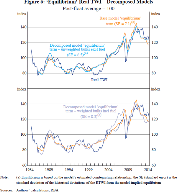
The estimated equilibrium from the unweighted narrow specification follows the observed RTWI more closely over the full sample than the estimated equilibrium from the baseline model. This is demonstrated by the slightly lower standard error (SE), which is a standardised measure of the observed RTWI's deviations from the estimated equilibrium. In particular, it tracks the RTWI more closely in 2008 and since 2013.
In contrast, the estimated equilibrium from the weighted broad specification diverged from the observed RTWI in 2013–14. However, given that this specification's equilibrium has a relatively poor fit over the entire sample, as indicated by the higher SE, the estimated deviation in 2013–14 does not appear to have been especially unusual in the context of this model. While the higher SE indicates a poorer fit, it only provides a simple benchmark for assessing the models, and other factors – including the theoretical soundness of the model – should also be considered in evaluating their usefulness. In particular, this specification arguably provides the purest decomposition of the ToT into bulks and excluding-bulks (in that it encompasses the full range of bulk commodities and accounts for changing export shares).
Overall, while there is some evidence that bulk commodity export prices have a smaller effect on the RTWI than other export prices, including separate variables in the model to directly capture this has only a small effect on the models' explanatory power over the full sample period. Moreover, including separate variables also leads to model specifications that are less parsimonious than the baseline model, and to estimated equilibriums that are quite sensitive to the exact model specification.
5.1.2 Is investment a better indicator of the effect of higher bulks prices?
As discussed above, the structure of the bulks industry means that a sizeable portion of the income associated with an increase in bulk commodity export prices will flow overseas and so the direct effect on domestic demand, relative prices and the RTWI could be relatively limited. Nevertheless, a portion of the income is still likely to flow into the domestic economy, particularly if the higher prices are accompanied by an increase in (labour-intensive) investment in the bulks sector. The increased demand for labour associated with this investment could contribute to a real appreciation of the exchange rate by: pushing up relative wages and prices; and by increasing demand for Australian dollars to pay those wages, and thereby placing upward pressure on the nominal exchange rate.
However, the relationship between investment in the bulks sector and developments in bulk commodity prices can be variable, both in terms of its strength and its timing, in part reflecting the ‘lumpy’ nature of investment in the mining sector. Moreover, in the recent mining investment boom, at least a portion of the investment in the LNG sub-sector is likely to have reflected factors such as technological improvements, which have made projects more viable, rather than increases in current and/or expected future prices alone.
This variability could, in turn, weaken the apparent relationship between the ToT and the RTWI during certain periods. One intuitive example of this dynamic is that, even if the ToT were to remain elevated, the exchange rate could still be expected to depreciate as the resources boom moves from its ‘investment’ phase to its (less labour-intensive) ‘production’ phase due to the associated easing in labour demand and reduction in (the growth rate of) real wages.[30]
These considerations suggest that investment could potentially be a better indicator of the effect of higher bulks prices on the economy – and therefore on the RTWI – than the prices themselves. To examine this, an investment-to-GDP ratio (I/GDP) variable can be added to the model's cointegrating relationship:
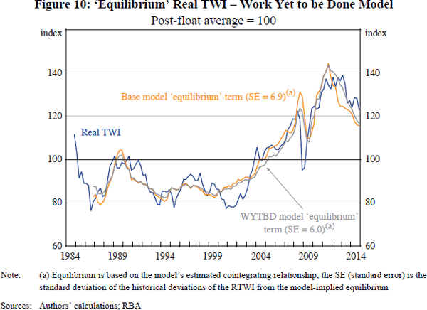
Two measures of I/GDP are considered. One is constructed using private business investment from the national accounts (Figure 7).[31] The other uses a forward-looking measure of non-residential construction work yet to be done (WYTBD) (Figure 8).
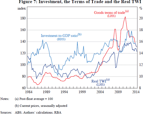
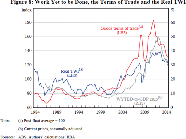
The results from incorporating the I/GDP variables into the baseline model are reported in Table 3.[32] The coefficients on both investment variables are positive, as expected, but only the coefficient in the WYTBD specification is statistically significant. At the same time, the coefficient on the ToT is lower in both models (relative to the baseline ECM). This could reflect the fact that these variants of the model allow the recent investment boom to have a direct effect on the exchange rate, whereas in the baseline ECM some of its effect may have been attributed to the higher ToT (i.e. omitted variable bias). However, there is some evidence of collinearity, which makes it difficult to interpret the magnitude and significance of the individual coefficients.
| Baseline | Investment | WYTBD | |
|---|---|---|---|
| Variables | |||
| Constant | 0.41** (0.11) |
0.43*** (0.11) |
0.65*** (0.17) |
| Speed-of-adjustment | −0.22*** (0.05) |
−0.23*** (0.05) |
−0.24*** (0.05) |
| Equilibrium relationships | |||
| Terms of trade | 0.59*** (0.05) |
0.53*** (0.06) |
0.39*** (0.09) |
| Real interest rate differential | 1.40 (1.04) |
1.56* (0.90) |
1.70** (0.83) |
| Total investment/GDP | 1.60 (1.09) |
||
| Work yet to be done/GDP | 0.48** (0.21) |
||
| In-sample fit statistics | |||
| R2 | 0.51 | 0.56 | 0.59 |
| Adjusted R2 | 0.48 | 0.51 | 0.54 |
| Out-of sample forecast statistics(a) | |||
| Clark-West bootstrapped | |||
| One-quarter horizon | 0.04 | 0.04 | 0.05 |
| Four-quarter horizon | 0.09 | 0.10 | 0.11 |
| Sixteen-quarter horizon | 0.20 | 0.24 | 0.37 |
| Diebold-Mariano bootstrapped | |||
| One-quarter horizon | 0.00 | 0.00 | 0.00 |
| Four-quarter horizon | 0.01 | 0.01 | 0.02 |
| Sixteen-quarter horizon | 0.12 | 0.10 | 0.24 |
|
Notes: The equations are estimated by ordinary least squares using quarterly data;
the Baseline and Investment equations are estimated over 1986:Q2–2014:Q4,
the WYTBD equation is estimated over 1986:Q4–2014:Q4; ***, ** and
* denote significance at the 1, 5 and 10 per cent levels, respectively;
standard errors are reported in parentheses (a) H0: forecast equivalence to a random walk; calculated using rolling windows |
|||
The models with the investment variables have slightly better in-sample fits than the baseline model; likelihood ratio tests suggest that these differences are statistically significant. Their out-of-sample forecast performance is similar to that of the baseline model, though the WYTBD model performs relatively poorly at the sixteen-quarter horizon.[33]
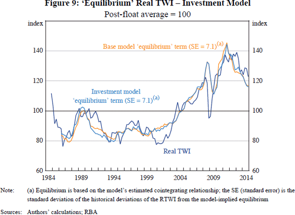
The estimated equilibrium terms from these models are fairly similar to the estimated equilibrium term from the baseline ECM (Figures 9 and 10). Nevertheless, there has been some divergence in recent years. In particular, the estimated equilibrium from the models that include the investment variables have tended to be higher than the estimated equilibrium from the baseline model, reflecting the continuing high levels of investment even after the ToT declined from its peak in 2011. This also means that the equilibriums from the models which include the investment variables have tracked the observed RTWI somewhat more closely during this latter period. Nevertheless, taken as a whole, the results are not very different to those from the baseline model, which is more parsimonious.
5.2 Bulk Commodity Prices and Expectations
Section 5.1 considered some reasons why the bulk commodities sector could interact differently with the economy than other sectors, which could help to explain why bulk commodity prices have a different effect on the RTWI than other export prices. A second potential reason why bulk commodity prices may have a different effect on the RTWI is that bulks prices may be less forward-looking and therefore contain less relevant information for foreign exchange market participants.
This second explanation may be important as a number of papers suggest that it is the expected path of the ToT that will affect domestic consumption, and therefore the exchange rate, through its influence on the expected path of future income (Chen et al 2010). For example, if agents expect an increase in the ToT – and the associated rise in domestic income – to be only transitory, they are likely to save a relatively high proportion of that income. In this scenario, the effect on domestic demand will be more muted than would be expected if the increase in the ToT was perceived to be persistent and the associated increase in income more permanent. Accordingly, we may expect a transitory ToT shock to be associated with less real appreciation pressure via the relative price channel than might be the case for a persistent ToT shock (all else equal). In a similar vein, forward-looking foreign exchange market participants should ‘price in’ expected changes in the ToT and ‘look through’ changes that are perceived to be only transitory, which suggests that there is also likely to be less nominal exchange rate appreciation than might be the case if the shock was perceived to be more long-lasting.[34]
There are several reasons why bulk commodity export prices, as measured in the ToT, could be less reflective of expectations of future demand and supply than other export prices. For example, until relatively recently, prices for bulk commodities were set predominantly using long-term contracts. While these contracts should incorporate expectations at the time they are set, prices are not able to react immediately to subsequent changes in the outlook for future supply and demand. In contrast, the (nominal) exchange rate is likely to respond to these changes, which could contribute to divergences between the ToT and the RTWI. This dynamic was particularly evident in late 2008, when a number of contracts for bulk commodity exports were agreed just before the onset of the (unanticipated) global financial crisis. While the nominal exchange rate – and therefore the RTWI – depreciated immediately, bulk export prices – and therefore the ToT – did not decline immediately.
More recently, the shift towards the use of shorter-term contracts and spot pricing for bulk commodities has reduced some of this price stickiness. Nevertheless, bulks prices are still likely to be less reflective of expectations than some other prices – at least periodically. This is because bulk commodities markets can be prone to transitory price spikes, reflecting relatively inelastic supply as well as the tendency for natural disasters to cause supply disruptions. Market participants and, consequently, the exchange rate are likely to ‘look through’ such price spikes, which can contribute to temporary divergences between the ToT and the RTWI. One prominent example of this dynamic occurred in 2010–11, when floods in Queensland pushed coal prices and the ToT higher, while the RTWI remained relatively unchanged.
Together, these factors suggest that a forward-looking measure of the ToT, which incorporates expectations for future bulk (and non-bulk) commodity export prices, could exhibit a stronger and more consistent relationship with the RTWI than the backward-looking observed ToT.
5.2.1 Is the exchange rate more responsive to a forward-looking terms of trade?
To investigate the relationship between the RTWI and the expected ToT, a number of forward-looking measures of the ToT were constructed using past vintages of the RBA's internal goods and services ToT forecasts.[35] The measures were constructed using forecast horizons of 4–8 quarters ahead for a sample beginning in 2003. The exercise assumes that the Bank's forecasts provide a reasonable proxy for the market's expectations for the ToT, which is, in turn, the relevant determinant of the exchange rate.[36]
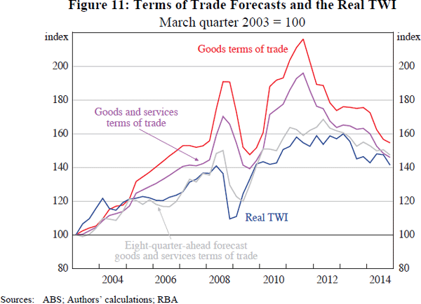
As expected, this forward-looking ToT measure appears to track the RTWI more closely than the observed ToT (Figure 11). This is particularly evident in 2008, when both the forward-looking ToT and the RTWI appear to have declined more quickly in response to the onset of the global financial crisis than the observed ToT. Similarly, both the forward-looking ToT and the RTWI appear to have ‘looked through’ the Queensland flood-induced spike in the observed ToT in 2010–11.
In order to formally test the relationship between expectations for the ToT and the RTWI, various forward-looking ToT measures (FToTs) are included in the cointegrating relationship of the baseline model in place of the observed ToT:[37]
The results from the model that includes an eight-quarter-ahead ToT forecast variable are reported in Table 4 (other forecast horizons were also considered, with similar results). As expected, when both models are estimated over a sample beginning in 2003, the speed-of-adjustment coefficient from the forward-looking model is larger (in absolute terms) than the speed-of-adjustment coefficient from the baseline model, suggesting that the RTWI responds more quickly to changes in the FToT than the observed ToT.[38] The in-sample fit of both the baseline and the eight-quarter-ahead models is similar.[39]
| Baseline | Eight-quarter-ahead | |
|---|---|---|
| Variables | ||
| Constant | 0.55*** (0.15) |
0.66*** (0.15) |
| Speed-of-adjustment | −0.24*** (0.06) |
−0.48*** (0.11) |
| Equilibrium relationships | ||
| Terms of trade | 0.50*** (0.07) |
0.72*** (0.05) |
| Real interest rate differential | 1.24 (1.93) |
0.28 (0.91) |
| In-sample fit statistics | ||
| R2 | 0.85 | 0.87 |
| Adjusted R2 | 0.82 | 0.84 |
| Notes: The equation is estimated by ordinary least squares using quarterly data; ***, ** and * denote significance at the 1, 5 and 10 per cent levels, respectively; standard errors are reported in parentheses | ||
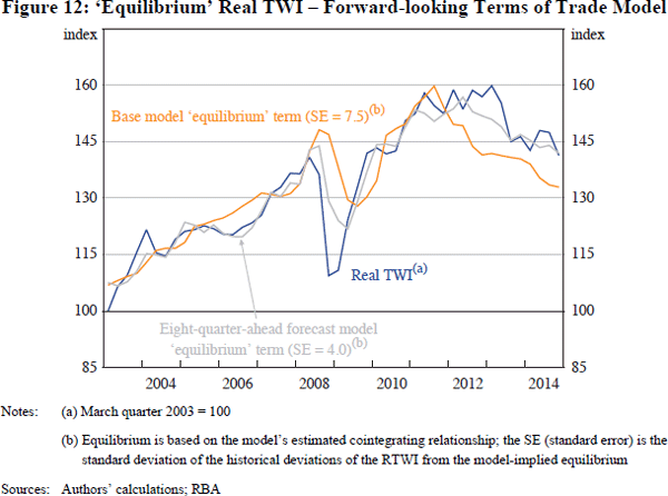
The estimated equilibrium from the FToT model tracks the observed RTWI more closely than the estimated equilibrium from the baseline model (when it is estimated over the same shorter sample period), as evidenced by the smaller SE (Figure 12). This is particularly evident in 2008 and also between 2012 and end 2014. Overall, the results suggest that the RTWI may display a more robust relationship with a forward-looking measure of the ToT, albeit over a significantly shorter sample period than the baseline model.
Footnotes
For more information on the ToT boom and its implications for the Australian economy see, for example, Connolly and Orsmond (2011), Plumb et al (2013), Sheehan and Gregory (2013), Atkin et al (2014) and Downes, Hanslow and Tulip (2014). [26]
Unit root tests indicate that the decomposed ToT series are also non-stationary over the sample. [27]
A similar approach was used to model the Canadian dollar in Maier and DePratto (2008). [28]
For details on the out-of-sample forecast testing procedures, see Appendix A. [29]
Debelle (2014) suggests a similar dynamic. As the investment phase ends, foreign firms will require fewer Australian dollars to pay for Australian inputs. At the same time, the increased production will not (directly) lead to much additional demand for Australian dollars as bulk commodities tend to be priced in US dollars, though there will still be some additional demand due to the higher dividends and taxes associated with increased production. Overall though, the net demand for Australian dollars is still likely to be reduced. [30]
A measure of mining investment was also considered, but the estimated coefficients were insignificant. Moreover, a likelihood ratio test suggested that including the mining investment variable did not significantly improve the fit of the model. [31]
Unit root tests indicate that both investment variables are non-stationary over the sample. [32]
Evidence of strong exogeneity is more mixed for the WYTBD variable, suggesting that the multi-step-ahead forecasting results should be interpreted with caution. [33]
The importance of considering expectations when examining the relationship between the ToT and the RTWI has been well documented for Australia. For example, Blundell-Wignall et al (1993) and Tarditi (1996) identify the early 1980s as a period when the RTWI appreciated in response to expected future increases in the ToT, which never eventuated. [34]
The goods ToT is used in the baseline ECM due to concerns over endogeneity between the RTWI and the services ToT (see Stone et al (2005) for details). However, this potential endogeneity problem will not be an issue when using forecasts for the ToT given that these forecasts are determined before the RTWI is known. [35]
A time series of market forecasts for the ToT is not readily available. [36]
Unit root tests indicate that the FToTs are non-stationary over the sample. [37]
Illustrative analysis suggests that this is also the case when the other short-run dynamics are included. [38]
Out-of-sample forecast statistics were not calculated due to the short length of the sample. [39]


