RDP 2018-04: DSGE Reno: Adding a Housing Block to a Small Open Economy Model 6. Housing and Australia's Post Mining Boom Transition
April 2018
- Download the Paper 1,668KB
In this section, we use the model to assess the role of housing investment in supporting economic activity since the end of the mining boom in 2012. The DSGE model provides us with two ways to assess how important activity in the housing sector was in helping the rebalancing of the economy. The first is to use a historical decomposition to quantify how much of the recent increase in housing investment is related to lower commodity prices, and in particular to lower interest rates associated with these lower prices. The second is to run a counterfactual scenario where housing sector activity does not pick up after the end of the mining boom.
6.1 Historical Decomposition
The idea behind a historical decomposition is as follows. The model attributes all deviations of the observable variables from their steady-state values to the model's structural shocks. A historical decomposition recovers these shocks and therefore allows us to single out which structural shocks have been driving a given variable of interest.
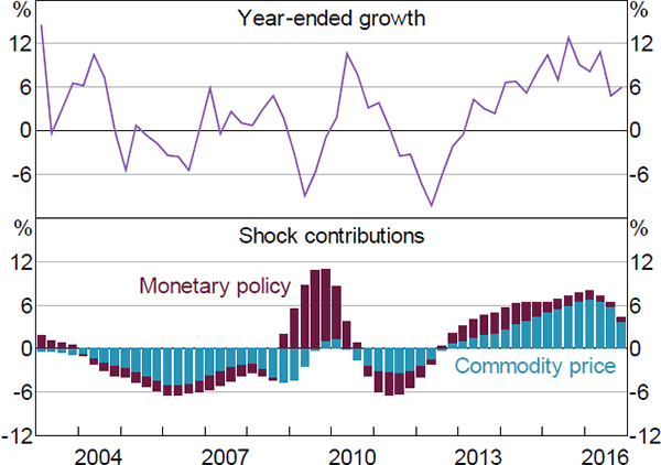
The model interprets fluctuations in commodity prices over the cycle as a series of positive and negative commodity price shocks. In order to examine the response of housing investment to the end of the mining boom we therefore focus on commodity price shocks.
In the model, a key channel through which commodity price shocks affect housing investment is by influencing interest rates. As commodity prices fall, disinflationary pressures lead the central bank to lower interest rates, which in turn stimulates housing investment.[24] We refer to this effect as the ‘endogenous’ interest rate channel. This channel reflects how the central bank responds to broader macroeconomic consequences of the fall in commodity prices, that is, falls in inflation, output, and employment. To the extent that the central bank takes other factors into consideration, this will show up in the model as monetary policy shocks.
Commodity price shocks consistently weighed on housing investment during the 2000s and continued to do so until the peak of the terms of trade in 2012 (Figure 16). This reflects the endogenous response of interest rates to the expansionary impulse, and more generally the flow of inputs towards mining activities and investment. More recently, as commodity prices have fallen, the opposite forces have been at work. This is consistent with the notion that housing investment has stepped in to fill the void left by the mining boom and to assist in the economic transition.
Meanwhile, monetary policy shocks have consistently made positive contributions to housing investment since 2013. This indicates that monetary policy has been looser than the model predicts based on its estimated relationships and the observables. In this sense, monetary policy has provided additional help in the transition of the economy. We note, however, that in recent years the independent contribution of monetary policy shocks has declined relative to that of commodity price shocks. One potential explanation for these dynamics is that monetary policy is more forward looking than is implied by the model specification. To the extent that policymakers expected future declines in commodity prices to weigh on future inflation and growth, they may have responded pre-emptively. The model would interpret this pre-emptive action as monetary policy shocks, even if it was related to (future) commodity price shocks.
Taken together, the above results suggest that the housing investment boom we have observed in recent years was largely a ‘natural’ response of the Australian economy to the large fall in commodity prices. Even in the absence of all monetary policy shocks, the model still predicts large increases in housing investment as a response to the end of the mining boom.
Sources: ABS; Authors' calculations
In this context, it is also worth considering the role of other shocks in the evolution of housing investment. Aside from commodity price and monetary policy shocks, the model also suggests that housing investment shocks have played an important role in determining housing investment in recent years. However, somewhat surprisingly the model suggests that housing investment shocks have weighed on housing investment. That is, housing investment has been somewhat weaker than the model would predict given the prevailing macroeconomic conditions. One potential explanation could be capacity constraints in the housing construction industry, which the (linear) model is not able to adequately capture. It is also possible that changes in lending standards could have weighed on investment.
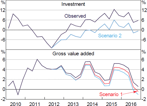
6.2 Counterfactual Scenario
As noted above, another way to assess the importance of the housing sector in aiding Australia's economic transition is to use a counterfactual scenario. Specifically, we run a scenario where housing investment and value added continued growing at their mining boom averages, rather than accelerating. For the counterfactual, we define the mining boom as March quarter 2003 to June quarter 2012.
We start by taking the structural shocks estimated using a historical decomposition, discussed above. With these shocks in hand, we can then look at our counterfactual while incorporating all of the shocks that would have hit the economy over the period.
Table 7 shows the averages of quarterly growth in housing investment and housing sector value added over the boom and post-boom periods. We use these averages to produce two different scenarios. In the first, we lower quarterly housing investment growth by 1.6 percentage points for each quarter in the post-boom period. We do so using shocks to housing investment. In the second, we also incorporate housing sector-specific technology shocks so that quarterly growth in housing sector value added is, on average, 0.2 percentage points below its actual history.[25],[26] The resulting calibrations for these scenarios are shown in Figure 17 (note housing investment is the same in scenarios 1 and 2).
| Housing investment | Housing sector value added | |
|---|---|---|
| Boom: 2003:Q1–2012:Q2, per cent | 0.0 | 0.6 |
| Post-boom: 2012:Q3–2016:Q4, per cent | 1.6 | 0.8 |
| Difference, percentage points | 1.6 | 0.2 |
Sources: ABS; Authors' calculations
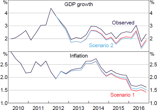
Figure 18 compares the observed growth in GDP and inflation to our scenarios. Under the scenarios, year-ended GDP growth is around ½ percentage point lower. Inflation is also somewhat lower; however, disinflationary pressures from softer growth are partly offset by higher inflation in the housing sector due to the smaller and less productive housing stock. Under both scenarios, the cash rate is around 40 basis points lower.
Sources: ABS; Authors' calculations
These estimates potentially understate the importance of the housing sector in the economy's transition. The model does not include borrowing, and therefore cannot account for any loosening of collateral constraints associated with the strong housing price growth witnessed in some cities over recent years. Similarly, as we model the price of housing services, not of the housing stock, the model may not adequately account for wealth effects associated with said housing price growth. Moreover, the model assumes that all investment is done using the final consumption good. This does not allow the inputs into different types of investment to differ. To the extent that the inputs used in mining investment are more similar to those used in residential construction than to those used in (for example) machinery and equipment investment, the housing sector may play a more important role in smoothing the economy's transition away from mining than the model indicates.
Footnotes
Jääskelä and Smith (2013) find that increases in the terms of trade are not always associated with inflationary pressures and higher interest rates. Our commodity price shock is most similar to their world demand shock, which is associated with higher domestic interest rates. [24]
As these housing technology shocks weigh on housing investment, the housing investment shocks required to hit our target for housing investment are smaller than in scenario 1. [25]
We choose technology shocks as apartments have made up a particularly large portion of recent residential construction (e.g. Shoory 2016). In some sense, this can be seen as a positive technology shock, as a given amount of investment produces more dwellings and housing services compared to construction of single-family dwellings. This type of interpretation is supported by the historical decomposition, which shows that improved productivity in the housing services sector has supported value-added growth. [26]