RDP 2018-04: DSGE Reno: Adding a Housing Block to a Small Open Economy Model 4. The Transmission of Monetary Policy
April 2018
- Download the Paper 1,668KB
This section compares the transmission of monetary policy in our model to RSH.[19] This allows us to quantify the differences in dynamics that come from the addition of the housing sector and the changes to household preferences. To this end, we use a modified version of RSH that includes our sticky wage specification, inflation indexation, and the same foreign sector as we consider in this paper.
4.1 Impulse Responses to a Monetary Policy Shock
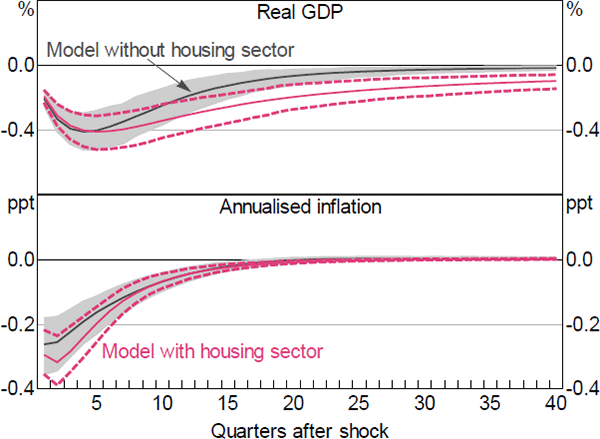
Figure 9 shows the responses of real GDP and inflation to a 100 basis point increase in the cash rate. Tighter monetary policy leads to a contraction in the real economy. GDP decreases by around 0.4 per cent at its peak, which occurs five quarters after the shock. The decline in GDP, which is within the range of estimates from empirical VAR models (e.g. Berkelmans 2005; Lawson and Rees 2008), is more persistent in our model than in RSH (the model without housing). This reflects more persistent declines in both consumption and investment. The increase in the cash rate lowers inflation slightly more than in the RSH model.

Note: 100 basis point increase in cash rate
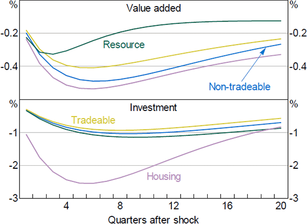
Figure 10 shows the responses of sectoral investment and value added in our model. These provide some insight into the model dynamics. Consistent with SVAR evidence we present below, the housing sector is the most interest-sensitive sector – particularly housing investment, which declines by around 2.5 per cent, similar to Lawson and Rees (2008). Meanwhile, value added in the resource sector is the least responsive, reflecting the fact that conditions in the sector are heavily influenced by foreign, rather than domestic, developments.
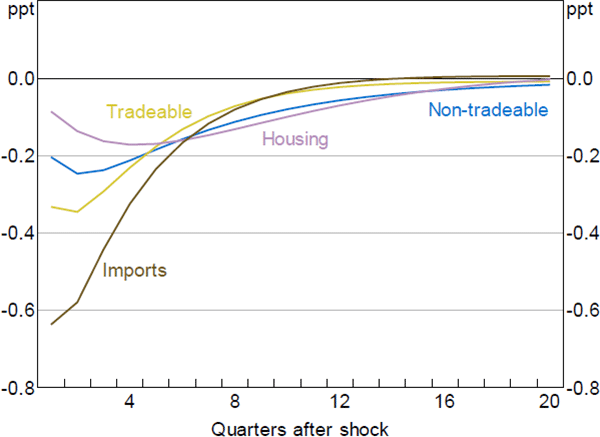
Figure 11 shows the response of sectoral inflation to the monetary policy shock. Housing services inflation has the smallest but the most persistent response. While this seems somewhat at odds with the fact that housing investment and output are reasonably sensitive to changes in the cash rate, the muted response of housing services inflation reflects two offsetting factors. On the one hand, lower aggregate demand places downward pressure on the price of housing services. On the other hand, the large fall in housing investment, and associated decrease in the housing stock, places upward pressure on prices. Thus, the overall response of housing services inflation is muted. Conversely, the price of imported goods and services declines substantially on impact. This is mainly due to the exchange rate appreciation induced by higher interest rates. Inflation decreases mildly in the tradeable and non-tradeable sectors.

Note: 100 basis point increase in cash rate

Note: 100 basis point increase in cash rate
4.2 Empirical Evidence from SVARs
As shown above, our model and RSH have slightly different dynamic predictions. This raises two related questions:
- To what extent are these differences a natural consequence of analysing more disaggregated data?
- To the extent that they reflect modelling choices, do our modelling choices help us to match the observed data?
We attempt to answer these questions by studying the dynamics implied by the more disaggregated data in a much less structured environment – SVARs. In particular, we estimate a series of SVARs using a subset of the same data we use in estimating the DSGE model and compare the impulse responses implied by the SVARs to those implied by the DSGE model.
4.2.2 The SVAR model
We assume that the economy can be represented using the following structural form:
where the matrix B summarises the contemporaneous relationships between the variables; C(L) is an autoregressive lag polynomial of order L, which summarises how the variables are affected by their own lags as well as the lags of the other variables in the system; and ut is a vector of independently and identically distributed structural shocks. The vector Xt contains foreign and domestic variables. We assume that the foreign variables are block exogenous: domestic variables cannot affect the foreign variables either contemporaneously or with a lag. This is consistent with other SVAR models of the Australian economy, where Australia is modelled as a small open economy (e.g. Manalo, Perera and Rees 2014). The foreign variables are the same ones we include in the DSGE model: commodity prices ( ); a measure of global economic activity (
 ); the average foreign inflation rate (
 ); and the average foreign policy rate (
 ). The domestic variables mimic a cut down version of the domestic economy from the DSGE model, and include: a set of GDP components (discussed below) denoted by
  ; trimmed mean inflation (πt); the cash rate (rt); and the real trade-weighted exchange rate (qt). Thus, the full vector
  .
.
As in the DSGE model, all variables are quarterly growth rates except the foreign and domestic policy rates, which are expressed in percentage points, and the sample runs from 1992:Q1 to 2016:Q4. We include three separate dummy variables in the model to account for: the introduction of inflation targeting (1992:Q1–1992:Q4); the introduction of the goods and services tax (2000:Q2–2000:Q3) and the global financial crisis (2008:Q4–2009:Q3). Considering the large number of variables included in the model, and for consistency across the results, we estimate all specifications with two lags (Liu, Pagan and Robinson (2018) show that such a lag length is sufficient to capture the dynamics of the RSH model).
We identify monetary policy shocks using a recursive ordering approach, where each variable in Xt can contemporaneously affect only variables later in the ordering.[20] Our ordering implies that shocks to real activity and inflation contemporaneously affect the cash rate. However, changes in the cash rate affect the other macroeconomic variables with a lag. This is a standard identification assumption of monetary policy shocks and reflects that fact that it takes time for economic agents to alter pricing, production and spending decisions in response to changed monetary policy conditions.[21]
4.2.3 SVAR results
We estimate four separate SVARs, which differ from each other in the way in which we decompose aggregate output growth. Specifically, we decompose aggregate output growth either into its expenditure components or into gross value-added production in the different sectors of the economy. For both decompositions, we estimate one SVAR where we separate out housing, and one where we do not. The GDP components included in each specification are summarised in Table 6.
| Model | Components |
|---|---|
| Model 1 | Tradeable sector value added, non-tradeable sector value added, resource sector value added |
| Model 2 | Tradeable sector value added, non-tradeable sector (excluding housing) value added, housing sector value added, resource sector value added |
| Model 3 | Consumption, investment, exports, imports |
| Model 4 | Consumption, investment (excluding housing), housing investment, exports, imports |
The models that separate out housing are similar in structure to our DSGE model, while the models that do not split out housing are similar in structure to the model in RSH. Therefore, by comparing the responses of the variables to a monetary policy shock across the SVAR models, we can gauge the importance of explicitly accounting for the housing sector. Moreover, we can also assess whether our assumption that housing investment is more interest sensitive is borne out in the data.
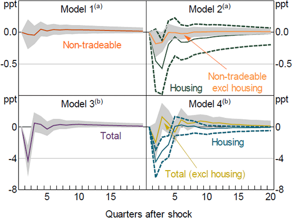
Figure 12 shows the responses of selected variables to an exogenous 100 basis point increase in the cash rate, along with the 68 per cent confidence bands. In Model 1, the response of value-added growth in the non-tradeable sector is very small and is not statistically significant. However, if we split the housing sector out, as we do in Model 2, the negative response of growth in value added for the non-tradeable (excluding housing) sector is larger and more persistent, although still not statistically significant. Value-added growth in the housing sector declines by almost 0.6 percentage points. Although the confidence intervals around this response are wide, the decrease in housing value-added growth is statistically significant after two quarters.

Notes:
100 basis point increase in cash rate
(a) Sector value added
(b) Investment
While it might seem surprising that the responses are larger for both sectors in Model 2, the finding is broadly consistent with Lawson and Rees (2008). They estimate an SVAR of the Australian economy including the expenditure components of GDP, and find that the implied aggregate response of GDP from this model is larger and more persistent than the response from a model estimated using aggregate GDP (in place of the expenditure components). Both sets of findings suggest that aggregating across sectors leads to a loss of useful information, which reinforces the importance of separately modelling the housing sector in the DSGE model.
Looking at the models that include the expenditure components of GDP, using Model 3 we find a statistically significant decline in total investment growth of about 4 percentage points in response to the monetary policy shock. However, if we decompose total investment into the housing and total excluding housing components, as we do in Model 4, it is evident that the aggregate response is largely driven by dwelling investment. This is consistent with the dynamic predictions of our model, and supports our decision to calibrate investment adjustment costs in the non-housing sectors to be relatively high.
It is worth noting that while the SVAR results are qualitatively similar to those from the DSGE model, quantitatively there are some substantial differences. In particular, the responses of housing investment and value added are much larger in the SVAR. However, given the large confidence bands around the SVAR's estimated responses, as well as the simple identification scheme used, we prefer to focus on the qualitative results.
Footnotes
In Appendices B and C we compare the responses between the two models for commodity price and exchange rate shocks, respectively. [19]
For an overview of different methods for identifying monetary policy shocks, see Ramey (2016). [20]
As pointed out by our referees, our DSGE model is unlikely to be recursive. This means that there isn't a direct mapping from our DGSE model to the SVAR model specified in this section. We note, however, that our intent is not to estimate the VAR representation of our DSGE model. Rather, our aim is to show that the DSGE model results are consistent with evidence arising from a much less structured model. We do not explore alternative VAR identification strategies, such as sign restrictions, as our exercise here is intended to be illustrative. [21]
