RDP 2019-08: The Well-meaning Economist 2. Quasilinear Means Generalise Arithmetic Ones
September 2019
- Download the Paper 2,045KB
The concept of arithmetic mean is central to this work and will be familiar to readers already. To clarify notation, it is the ‘functional’ defined by
where: denotes the arithmetic mean of a discrete random variable Y ; X is a random vector of conditions; yi denotes a possible outcome of Y; and prob(Y = yi|X) is a conditional outcome probability function.
When Y is a continuous random variable,
where p(y|X) is a conditional probability density function for Y.
So the arithmetic mean described here is a population concept, not a sample one. And strictly speaking it is a conditional arithmetic mean, which includes the unconditional type as a special case. Usually I will omit these distinctions. Other names are average, first moment, and expectation. In theory, the arithmetic mean is undefined for some distributions, like the Cauchy case. In practical economic applications these distributions are uncommon, so wherever appears in this paper I assume it to be defined.
The concept has been used since the mid 1600s, with intellectual origins that are outlined in Ore (1960). By no later than Whitworth (1870) it was a textbook idea and today much of the standard economics toolkit builds around it. At the same time, the field has made practically no deliberate use of options from the broader quasilinear family of means, which are functionals of the form
Here Y is a discrete or continuous random variable and f (·) is a function that is continuous and strictly monotone over the domain of Y.[2] This concept has a shorter intellectual history, with origins in the 1920s (Muliere and Parmigiani 1993). It will be unfamiliar to most readers.
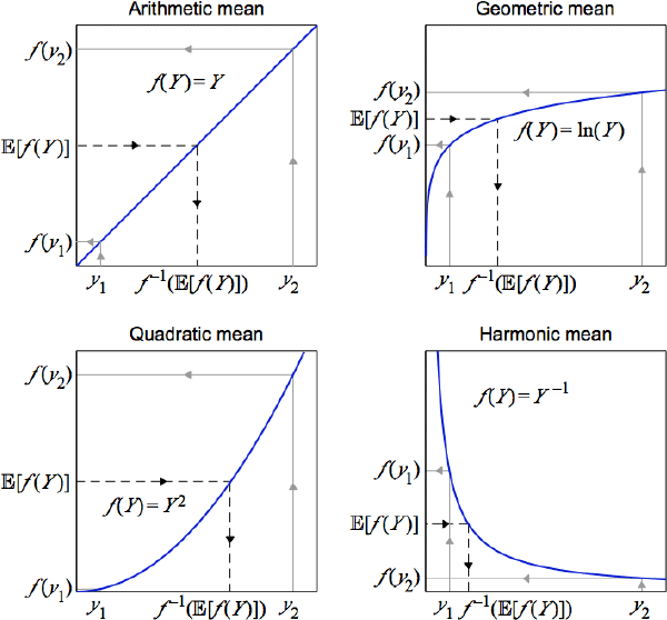
To illustrate the mechanics, a simple setting to consider is a random variable Y that takes only two possible values, y1 and y2, with equal probability. To calculate the quasilinear mean of Y, the two values are first mapped onto another space using a choice of f (·), like one of the four choices in Figure 1. An arithmetic mean of the two new values is then calculated using the respective outcome probabilities. Mapping this arithmetic mean back onto the original space produces the quasilinear mean of Y.

Different choices for the curvature of f (·) generate the specific cases. Emphasis is on curvature because each f (·) is unique only up to an affine transformation , where and are both constants and A notable specific case uses f (Y) = Y, which defines the arithmetic mean. Hence one of several alternate names for quasilinear mean is quasi-arithmetic mean.[3] Some other notable specific cases use: f (Y) = ln(Y), which defines the geometric mean; f (Y) = Y–1, which defines the harmonic mean; and f (Y) = Y2, which defines the quadratic mean.
Two other types of f (·) come up in this paper but not in the literature on quasilinear means. The first is the inverse hyperbolic sine (IHS) transformation, f (Y) = log(Y + (Y2 + 1)1/2), or sometimes just f (Y) = sinh–1(Y). The second is where is a small and strictly positive constant. I will call this a gamma-shifted-log (GSL) transformation, and denote it with gsl(Y). Both types define quasilinear means that I will show relate to common econometric approaches.
Quasilinear means have properties that are excellent for the policymaker. Section 5 will discuss them in some detail.
Footnotes
Computer scientists already use a range of quasilinear means for machine learning, but not as features of an outcome distribution to learn about. Instead they use the means to summarise explanatory variables. See James (2016, Ch 5) for an illustration. [2]
Other names are generalised f-mean and Nagumo-Kolmogorov mean, after contributions in Nagumo (1930) and Kolmogorov (1930). [3]