Research Discussion Paper – RDP 2021-02 Online Appendix: Star Wars at Central Banks
Adam Gorajek, Joel Bank, Andrew Staib, Benjamin Malin and Hamish Fitchett
February 2021
This appendix provides additional information to accompany Research Discussion Paper No 2021–02
1. Extra Analysis for the p-curve
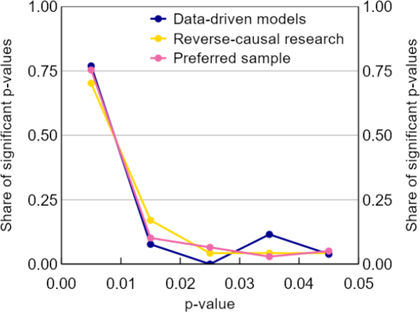
We find no statistical evidence of researcher bias in all of the subsamples we assess using the p-curve. In each case the p-curve decreases over p (Figure A1).

Sources: Authors' calculations; Federal Reserve Bank of Minneapolis; Reserve Bank of Australia; Reserve Bank of New Zealand
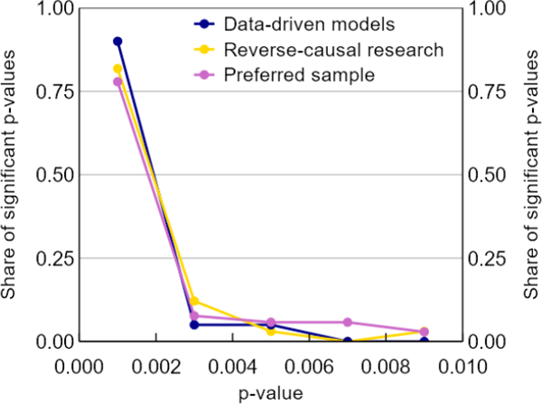
We also construct p-curves for these subgroups on a narrower window of significant results (p < 0.01) to account for the possibility of aggressive researcher bias. Simonsohn, Simmons and Nelson (2015) explain that if researcher bias is aggressive, in that it pushes results well beyond the 5 per cent significant threshold, the identifying assumptions of the p-curve are invalidated. To handle this possibility, they propose focusing on a narrower window of significant results. The results are the same (Figure A2).

Sources: Authors' calculations; Federal Reserve Bank of Minneapolis; Reserve Bank of Australia; Reserve Bank of New Zealand
Unsurprisingly, for our two main samples, we fail to formally reject the null of a uniform p-curve against the one-sided alternative that it slopes upwards (Table A1; we include this trivial result only because it was in our plan).
| Central bank | Top journals | ||||
|---|---|---|---|---|---|
| p = [0.00, 0.05] | p = [0.00, 0.01] | p = [0.00, 0.05] | p = [0.00, 0.01] | ||
| z-score | −48.45 | −50.90 | −74.99 | −78.52 | |
| Degrees of freedom | 185 | 137 | 623 | 445 | |
| p-value | 1 | 1 | 1 | 1 | |
|
Notes: The z-scores presented are the results from applying ‘Stouffer’s method’ as described in Kim et al (2013). The method is commonly used for conducting meta-analysis hypothesis tests. Our pre-analysis plan erroneously labels the method as a chi-squared test. Sources: Authors' calculations; Brodeur et al (2016); Federal Reserve Bank of Minneapolis; Reserve Bank of Australia; Reserve Bank of New Zealand |
|||||
2. Extra Analysis for the z-curve
To understand these extra figures deeply, we recommend reading Brodeur et al (2016) in detail. The body of our paper outlines only the intuition of their method, in 4 main steps. Below we include which of those steps each analysis relates to. We have changed some of the figure labels to make those relationships clearer.
For the 3 central banks taken together, the sample form of P[z|disseminated] for z larger than 5 suggests several plausible options for bias-free P[z] (Figure A3; these panels relate to Step 2 of the z-curve).
![Figure A3: Sample Distributions of P[z|disseminated] and Plausible Bias-free Forms of P[z[]](images/figure-a3.gif)
Notes: Bars are frequencies of the absolute values of de-rounded t-statistics (very close to z-score equivalents) for results that are the subject of a comment in the main text of a paper. Based on the right tail of distribution, there are many potential candidates for bias-free forms of P[z].
Sources: Authors' calculations; Federal Reserve Bank of Minneapolis; Reserve Bank of Australia; Reserve Bank of New Zealand
All options for bias-free P[z] generate similar amounts of unexplained variation in observed P[z|disseminated]; the cumulated residuals peak soon after the 5 per cent significance threshold and have peaks of similar heights (Figure A4; these panels relate to Steps 3 and 4 of the z-curve method). The results are insensitive to whether we estimate the shape of P[disseminated|z] parametrically or non-parametrically.
![Figure A4: Unexplained Variation in P[z|disseminated] and Our Estimates for P[disseminated|z]](images/figure-a4.gif)
Notes: We present a scaled probability for the shape of P[disseminated|z] because we do not account for the normalising constant we dropped from Bayes' rule (so as to follow Brodeur et al (2016) closely). Our estimates would require a linear transformation before they can be interpreted as probablilities.
Sources: Authors' calculations; Federal Reserve Bank of Minneapolis; Reserve Bank of Australia; Reserve Bank of New Zealand
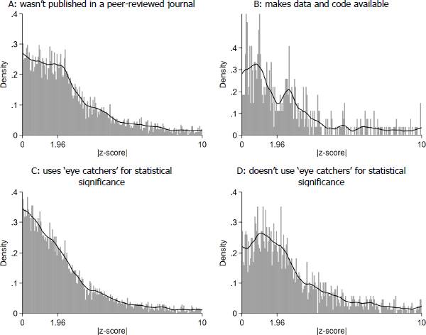
We had planned to produce z-curves for several subsamples not already presented in the paper (Figure A5). The sample sizes for several of these are quite small.

Notes: Plotted are the absolute values of de-rounded t-statistics (very close to z-score equivalents) for results that are the subject of a comment in the main text of a paper. We have also excluded results that come from data-driven model selection techniques or reverse causal research.
Sources: Authors' calculations; Federal Reserve Bank of Minneapolis; Reserve Bank of Australia; Reserve Bank of New Zealand
For all of our different subsamples (not just the ones shown above), the distribution of P[z|disseminated] for z larger than 5 suggests several plausible options for bias-free forms of P[z] (Figure A6; these panels relate to Step 2 of the z-curve method). The different subsamples don't all suggest the same bias-free forms of P[z].
![Figure A6: Observed Distributions of P[z|disseminated] and Plausible Bias-free Forms of P[z]](images/figure-a6.gif)
Notes: Bars are frequencies of the absolute values of de-rounded t-statistics (very close to z-score equivalents) for results that are the subject of a comment in the main text of a paper. We have also excluded results that come from data-driven model selection techniques or reverse causal research. Based on the right tail of the distributions, there are many potential candidates for bias-free forms of P[z]. The subsamples don't all suggest the same bias-free forms of P[z].
Sources: Authors' calculations; Federal Reserve Bank of Minneapolis; Reserve Bank of Australia; Reserve Bank of New Zealand
We had planned to use the controls as a sensible candidate for bias-free P[z]. In the end, however, the distribution of controls turned out to have far too much mass in the tails to meet the informal criteria in Step 2 of the z-curve method. The problem is so extreme that for insignificant z, P[z] is higher than P[z|disseminated], generating a maximum excess of results at low z (Figure A7). We find this result to be nonsense, and worry that it stems from our small sample size.
![Figure A7: Observed Distributions of P[z|disseminated] for Main Results against Controls](images/figure-a7.gif)
Notes: Bars are frequencies of the absolute values of de-rounded t-statistics (very close to z-score equivalents) for results that are the subject of a comment in the main text of a paper. The line curve is a kernel density for the corresponding test statistics on control variables. The distribution of controls has too much mass in the tails to meet the informal criteria in Step 2 of the z-curve method.
Sources: Authors' calculations; Federal Reserve Bank of Minneapolis; Reserve Bank of Australia; Reserve Bank of New Zealand
The subsamples all produce similar formal z-curve findings, but the results are not robust to sensible choices of bias-free P[z] (Table A2; these results relate to Step 4 of the z-curve method).
| Subsample | Input function used | Maximum cumulated residual | |
|---|---|---|---|
| Non-parametric estimate of P[disseminated|z] | Parametric estimate of P[disseminated|z] | ||
| Minneapolis Fed | Cauchy(1.5) | 2.0 | 1.6 |
| Cauchy(2) | 2.3 | 2.6 | |
| WDI | 1.6 | 1.1 | |
| VHLSS | 1.2 | 0.0 | |
| QOG | 1.2 | 0.2 | |
| RBA | Cauchy(1.5) | 2.9 | 3.0 |
| Student(1) | 1.4 | 2.5 | |
| WDI | 3.1 | 2.7 | |
| VHLSS | 3.1 | 2.0 | |
| QOG | 1.7 | 1.8 | |
| RBNZ | Cauchy(1.5) | 3.3 | 3.2 |
| Student(1) | 2.3 | 2.8 | |
| Published in a journal | Cauchy(1.5) | 2.6 | 2.4 |
| Student(1) | 1.4 | 2.1 | |
| WDI | 2.8 | 2.1 | |
| VHLSS | 3.0 | 1.5 | |
| QOG | 1.4 | 1.4 | |
| Not published in a journal | Cauchy(2) | 2.9 | 3.1 |
| WDI | 1.2 | 1.9 | |
| VHLSS | 1.2 | 1.5 | |
| QOG | 0.8 | 0.9 | |
| Uses ‘eye catchers’ | Cauchy(1.5) | 2.0 | 2.5 |
| Student(1) | 1.2 | 1.9 | |
| WDI | 2.0 | 2.2 | |
| VHLSS | 1.7 | 1.5 | |
| QOG | 0.9 | 1.4 | |
| Doesn't use ‘eye catchers’ | Cauchy(2) | 2.3 | 2.5 |
| WDI | 1.3 | 1.7 | |
| VHLSS | 1.5 | 1.5 | |
| QOG | 1.1 | 0.8 | |
|
Notes: The number 2.0 in the first column of data reads as ‘there is an unexplained excess of just-significant results that amounts to 2.0 per cent of all results’. The z-curve method attributes this excess to researcher bias. The different subsamples all produce similar formal z-curve findings. The assumed distributions for bias-free P[z] does matter somewhat though. Sources: Authors' calculations; Federal Reserve Bank of Minneapolis; Reserve Bank of Australia; Reserve Bank of New Zealand |
|||
References
Brodeur A, M Lé, M Sangnier and Y Zylberberg (2016), ‘Star Wars: The Empirics Strike Back’, American Economic Journal: Applied Economics, 8(1), pp 1–32.
Kim SC, SJ Lee, WJ Lee, YN Yum, JH Kim, S Sohn, JH Park, J Lee, J Lim and SW Kwon (2013), ‘Stouffer’s Test in a Large Scale Simultaneous Hypothesis Testing, PLoS One, 8(5), e63290.
Simonsohn U, JP Simmons and LD Nelson (2015), ‘Better P-curves: Making P-curve Analysis More Robust to Errors, Fraud, and Ambitious P-hacking, a Reply to Ulrich and Miller (2015)’, Journal of Experimental Psychology: General, 144(6), pp 1146–1152.