RDP 2021-03: Financial Conditions and Downside Risk to Economic Activity in Australia 3. How Do Financial Conditions Affect Risks to Economic Outcomes?
March 2021
- Download the Paper 1,967KB
We repeat the processes outlined in Section 2 using 5 measures of economic activity: real GDP growth, real household consumption growth, real non-mining business investment growth, employment growth and the change in the unemployment rate. Specifically, the distributions of future growth in each measure of economic activity are estimated using current growth in the relevant measure of economic activity, the FCI and a constant as explanatory variables. For each measure of economic activity the exercise is undertaken using both quarterly and year-ended changes to examine any possible differences in the near-term and longer-term effects of financial conditions on downside risk. Future work could examine longer time horizons, creating a ‘term structure of growth at risk’ as developed in Adrian et al (2018). Alternatively, we could compile a more detailed set of explanatory variables in order to better isolate the channels through which financial conditions influence economic risk.
Our main findings are:
- The FCI contains some useful information about different parts of the distribution of each of the 5 measures of economic activity we consider. This insight would be lost if we were to focus solely on the central tendency.
- The influence of financial conditions on the different measures of future economic activity tends to be asymmetric: the lower part of the distribution is often more variable than the upper part and the estimates of downside risk are more variable than the estimates of upside risk.
- Financial conditions are estimated to be a better predictor of future downside risk to GDP and employment growth (and upside risk to the unemployment rate) than they are of household consumption and business investment.
3.1 Estimated distributions of economic activity
We begin by looking at the QR model results to see if the coefficient estimates related to the FCI have different values for the different quantiles examined. This will provide evidence on whether the FCI is more important for explaining some parts of the distribution of economic activity than others. Figure 2 plots the coefficient estimates (columns) and 95 per cent confidence intervals (dashed lines) for the QR with real GDP and the FCI as the independent variables for = {0.05,0.25,0.50,0.75,0.95}.[16] The top row shows the coefficient estimates for quarterly growth in GDP while the bottom row shows the coefficient estimates for year-ended growth. For space reasons we will discuss the results for all 5 measures of economic activity in this section, but choose to only present figures for GDP and employment growth. All other figures are presented in Appendix B.
We find that the coefficient point estimates take on different values for the different quantiles considered, but the differences are not statistically significant. The coefficient estimate for the FCI at the median (0.5 quantile) is negative, indicating that more restrictive financial conditions in the current period tend to result in lower median GDP growth in the future for both quarterly and year-ended horizons. However, the coefficient estimates for the FCI associated with the tails of the distribution (i.e. the 0.05 and 0.95 quantiles) are positive. This indicates that tighter current financial conditions tend to widen the distribution of future GDP growth in both the left and right tails. This widening is more pronounced for the left tail of year-ended GDP growth than it is for quarterly GDP growth. Further, most of the coefficients on the lag of GDP growth are estimated to be smaller than the coefficients on the FCI, suggesting that current financial conditions are potentially more informative than current GDP growth in explaining the quantiles of future GDP growth.
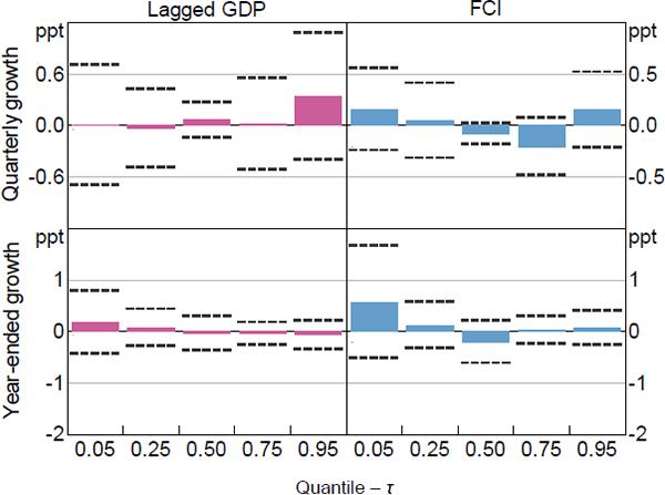
Note: Dashed lines represent 95 per cent confidence intervals computed using the stationary bootstrap proposed in Politis and Romano (1994) assuming an average block length of 8 quarters and 1,000 replications
Sources: ABS; Authors' calculations
The coefficient estimates for the other more granular measures of economic activity are broadly consistent with those for GDP growth. Generally, more restrictive current financial conditions have a negative relationship with the median future outcome for all the measures of activity (besides the unemployment rate which is, as expected, positive). However, among the other measures of economic activity, more restrictive current financial conditions only tend to widen the distribution for employment growth and the unemployment rate. In contrast, more restrictive current financial conditions tend to narrow the distribution of household consumption growth, and have a mixed effect on the upper and lower tails of the distribution of business investment (refer to Appendix B.1 for more detail).
The QR coefficient estimates can now be used to compute the fitted values of the QR model. These fitted values will in turn be used to generate the sequence of continuous PDFs and estimates of downside risks to economic activity. Figures 3 and 4 display the quarterly and year-ended fitted quantiles for GDP and employment growth.
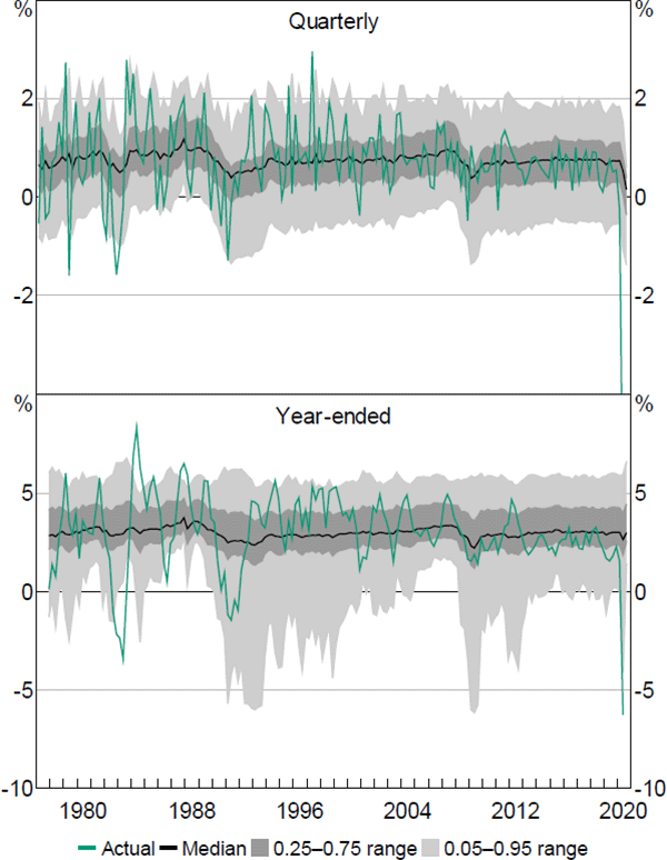
Notes: ‘GDP’ is the growth rate of real gross domestic product; actual quarterly growth rate for 2020:Q2 is –7 per cent
Sources: ABS; Authors' calculations
These figures show the estimated median, together with the estimated 0.25–0.75 and 0.05–0.95 quantile ranges for the fitted values of GDP and employment growth. The two figures highlight a key result: namely, that the outer part of the estimated distributions of both GDP and employment growth at both time horizons is more variable than the median. Further, in both cases there is also an asymmetric response. The lower parts of the estimated distributions are much more variable than the upper parts, especially for the year-ended horizon. This result is also found for the unemployment rate and, to a lesser extent, for household consumption and business investment. In the recent COVID-19 pandemic, the speed and depth of the contraction in economic activity during the March and June quarters of 2020 was far greater than that predicted by the quarterly versions of the QR model, highlighting the extreme, sudden and exogenous nature of the event. However, the year-ended estimates tended to fare much better (as the effect of June quarter 2020 is effectively ‘smoothed’), with the exception of household consumption (refer to Appendix B.2 for more detail).
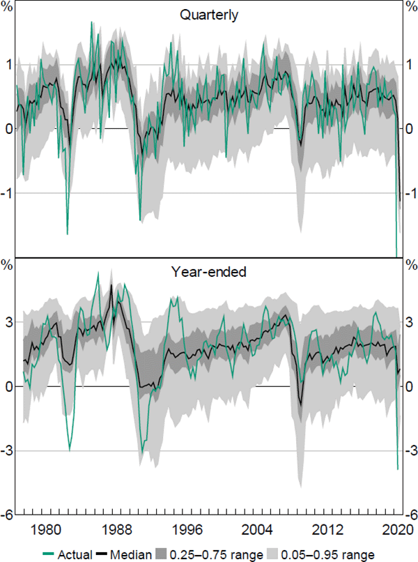
Notes: ‘Employment’ is the growth rate of total employment; actual quarterly growth rate for 2020:Q2 is –5 per cent
Sources: ABS; Authors' calculations
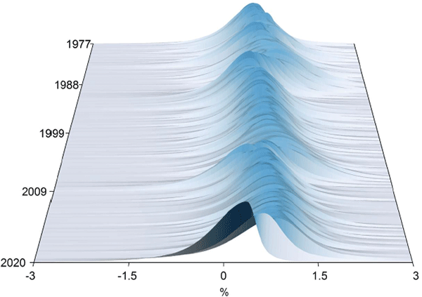
These findings underscore the benefit of modelling the entire distribution in circumstances when tail risk is of primary concern. Indeed, this result is even more evident when viewing the estimated sequences of PDFs produced from the fitted QR models for quarterly GDP growth over time (Figure 5).
Sources: ABS; Authors' calculations
The figure highlights that the location, scale and shape of the distribution for quarterly GDP growth all change over the sample period. The biggest changes occur around times of major downturns such as the 1982 recession, the 1989–91 recession, the GFC in 2008 and more recently the COVID-19 pandemic.
3.2 Downside and upside risks to economic activity
We now present the estimates of downside and upside risk to economic activity over both time horizons. These estimates are calculated as the area in the tails of the previously computed sequences of PDFs. In computing these measures of risk we employ a threshold quantile of = 0.05 for both horizons. The results for GDP growth and employment growth are displayed in Figures 6 and 7.
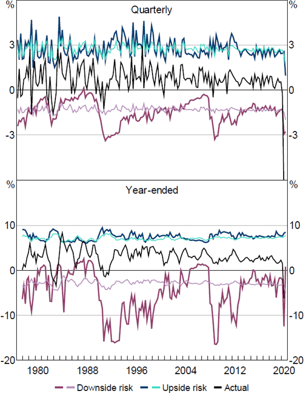
Notes: ‘GDP’ is the growth rate of real gross domestic product; actual quarterly growth rate for 2020:Q2 is –7 per cent; is set equal to 5 per cent; thicker darker-coloured line is estimated with the FCI; thinner lighter-coloured line is estimated without the FCI
Sources: ABS; Authors' calculations
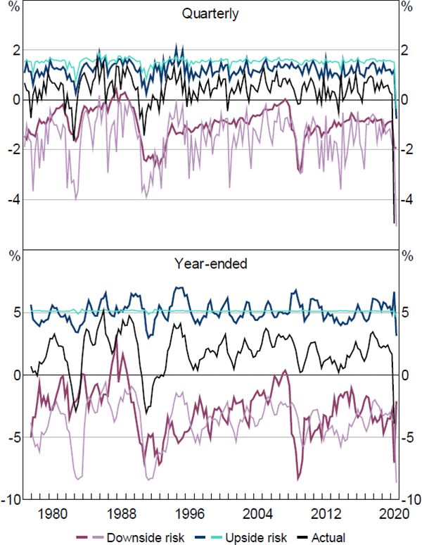
Notes: ‘Employment’ is the growth rate of total employment; is set equal to 5 per cent; thicker darker-coloured line is estimated with the FCI; thinner lighter-coloured line is estimated without the FCI
Sources: ABS; Authors' calculations
The ‘Downside risk’ lines show our estimate of what realised growth in either GDP or employment would have been if it was in the bottom 5 per cent of the fitted distributions at each point in time.[17] Similarly, the ‘Upside risk’ lines show our estimate of what growth in GDP or employment would have been if it was in the top 5 per cent of the fitted distributions at each point in time. The ‘Actual’ line represents the observed values for GDP growth and employment growth. For both downside and upside risk, the thicker darker-coloured lines signify the estimates obtained when both economic activity and financial conditions are included as explanatory variables in the QR model. In contrast, the thinner lighter-coloured lines signify the equivalent estimates when the FCI is excluded from the QR model and only current economic activity is used in estimation. As such, the difference between the thicker and thinner lines in each figure demonstrates the contribution that financial conditions make to the estimate of tail risk for that measure of economic activity.
The results show that estimates of downside and upside risk for GDP growth are much more variable when financial conditions are accounted for; especially around 1991–92 and 2008–09. This was also the case in the first half of 2020, with the model's estimates of downside risk to GDP growth performing relatively better in capturing the actual decline in GDP growth (at both horizons) than the estimates that exclude financial conditions as an explanatory variable. This suggests that the FCI contains useful information about downside risks to GDP growth, over and above measures of current GDP growth. For employment growth, however, the results indicate the FCI is more useful for explaining downside risks at a year-ended horizon than at a quarterly horizon.
The FCI also makes meaningful contributions to the estimates of upside risk to the unemployment rate (i.e. the risk of a large increase in unemployment), predominately at a year-ended time horizon. Downside risk is estimated to be more variable than upside risk for GDP and employment, while upside risk to the unemployment rate is estimated to be more variable than downside risk. In contrast, the aggregate FCI seems to make relatively little difference to the estimates of downside risk for household consumption and business investment, with the results for business investment also puzzling in that they display more variation in upside risk than they do in downside risk (refer to Appendix B.3 for detailed results for these activity measures). It is possible that more disaggregated measures of financial conditions could yield different results.
Overall, the results indicate that the ability of financial conditions to explain changes in downside risk to different measures of economic activity in Australia is mixed. For some series, financial conditions seem to provide useful additional information (i.e. GDP, employment and the unemployment rate) while for other series, financial conditions seem less informative (i.e. household consumption and business investment). It is possible that a model with more structure would allow us to more clearly identify the link between financial conditions and macroeconomic risk – including for variables like household consumption and business investment – however, this is beyond the scope of the GaR framework presented in this paper. Moreover, it is also important to note that because financial crises in Australia have been rare (in the period covered by our dataset there have only been two significant financial crises) the FCI's ability to contribute additional information about tail risk is likely to be limited to these two time periods.
Footnotes
The 95 per cent confidence intervals were constructed from bootstrapped standard errors using the stationary bootstrap developed in Politis and Romano (1994), assuming an average block length of 8 quarters and 1,000 replications. Note, we computed the standard errors in this way because the bootstrap methods proposed in Schmidt and Zhu (2016) ignore any potential serial correlation that might be present in the data. [16]
More specifically, it is the average of all estimated outcomes below the 0.05 quantile of the fitted distribution. [17]