RDP 2021-10: The Rise in Household Liquidity 5. Household Liquidity and Mortgage Debt Dynamics
November 2021
- Download the Paper 1.71MB
Taken together, the stylised facts indicate that there is a close link between the rise in household liquidity, the housing life cycle and the mortgage market. In this section, we outline the channels through which changes in household liquidity may be linked to changes in housing prices and debt.
To identify the channels through which mortgage debt, housing prices and household liquidity are related, we provide a conceptual framework based on a partial equilibrium two-period consumption model in Appendix D. Based on this framework, we outline each channel in turn and provide some testable predictions about the correlations between liquid assets, housing prices and mortgage debt which we take to the data:
- Housing deposit channel: households accumulate liquid assets for the deposit to purchase a home. This is typically around 10–20 per cent of the value of the home for a first home buyer. If this channel matters, we should observe a sharp decline in liquid assets at the time of first home purchase (as the buyer converts the liquid assets to housing equity). Assuming that housing prices continually rise, we should observe higher levels of liquidity prior to purchase over time and this effect should be particularly strong in more expensive housing markets, such as the large capital cities.
- Precautionary saving channel: home owners might increase their buffers for precautionary saving reasons, for example, because of increased uncertainty about future income or mortgage repayments. If precautionary saving matters, we should observe higher buffers for home owners that face greater income uncertainty, such as those that are more worried about losing their jobs or those that have more volatile incomes.
- Housing equity withdrawal channel: households can extract equity from their homes (at a cost) and this money can be consumed or saved in liquid assets, assuming they have positive home equity. A home owner can do this either by taking out a home equity loan or by selling their home and moving to a new home with less equity. Alternatively, home owners can refinance their mortgages to a lower interest rate to reduce the scheduled payment and free up money that can be consumed or saved in liquid assets. This channel predicts a positive correlation at the household level between the growth rate of debt and liquid assets at the time of equity extraction or refinancing.
5.1 The housing deposit channel
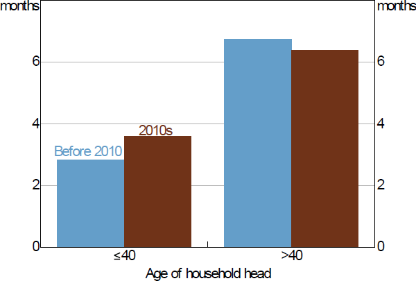
First, we consider whether the rise in household liquidity over time is connected to rising deposit requirements to purchase a home. If true, we should observe an increase in liquidity buffers among young renters – the households that are most likely to be potential first home buyers. We do find some evidence that buffers have increased among young renters (those with a household head aged less than or equal to 40 years) relative to older renters over the past decade (Figure 14).
But we can more closely identify the housing deposit channel by adopting an event study approach and examine what happens to liquidity when a household buys a home for the first time. For this, we need to track the liquidity position of a household before, during and after they purchase their first home, which requires longitudinal information from the HILDA Survey. We infer information on when each home owner bought their home, how much they paid for the home, and how much debt they took on at the time from the wealth modules (that are available every four years).[12]

Sources: ABS; Authors' calculations
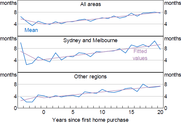
The event study indicates that, for those households that enter into home ownership, liquidity buffers are typically high in the years just prior to purchase, but drop sharply around the time of purchase, as the household converts their liquid savings to finance the deposit (Figure 15).[13] Following the purchase, the average new home owner gradually accumulates liquid wealth, but the level of buffer does not return to its pre-purchase level until at least 5 to 10 years after purchase.
The drop in liquidity at the time of first home purchase is also larger for households living in Sydney and Melbourne than elsewhere in the country. This is consistent with households in more expensive areas needing to save up more (or longer) for a deposit. Further, there are cohort effects in that first home buyers today start with higher levels of liquidity buffer prior to purchase than those first home buyers a decade ago. This suggests that rising housing prices have lifted the deposit requirement and this has played some role in explaining the trend increase in liquidity buffers.

Sources: Authors' calculations; HILDA Survey Release 19.0
5.2 The precautionary saving channel
In a world of uncertainty, indebted home owners may value liquidity for precautionary reasons, given the potential for future income falls or unexpected increases in interest rates. Rising levels of mortgage debt (relative to incomes) make the mortgage payments larger and the risk associated with any income or payment shock increases. Households may respond to this increased risk by increasing their rate of precautionary saving. The higher rate of saving can occur through both amortising mortgage debt (including paying ahead of schedule) and saving in other liquid assets, such as bank deposits and equities.
In this section, we examine the evidence that precautionary saving behaviour is important to explaining liquidity buffers amongst mortgagor households. For this, we construct two measures of household-level uncertainty.
First, we construct a forward-looking (subjective) measure based on the beliefs of working households about their future job prospects. The HILDA Survey directly asks workers for an estimate of the probability that they will lose their job in the year ahead. This subjective measure of job loss has been shown to have some predictive ability for actual job loss (Penrose and La Cava 2021). Workers are assumed to be more ‘uncertain’ the higher their subjective estimate of potential job loss is. This is referred to as the ‘forward-looking’ measure of income uncertainty. Workers that expect to lose their job are assumed to be more likely to engage in precautionary saving behaviour. We should therefore observe higher buffers among these households.
Second, a backward-looking (objective) measure is constructed based on the observed volatility of past household income. Households that have more volatile income streams are assumed to be more likely to save for precautionary reasons. The household-specific estimate of income volatility is constructed in a few steps. Household income is assumed to be a function of observable household-specific characteristics based on the following OLS regression model:
where the dependent variable is the log level of household disposable income ( yit ) and the determinants ( Xit ) include household-level characteristics such as a household head's age, education and whether they have a long-term health condition, as well as worker characteristics including job tenure, occupation, the nature of the labour contract (e.g. fixed or part-time basis) and the industry of work. From this regression model the residual income is estimated for each household and year . The standard deviation of this residual income is then constructed over rolling three-year windows to obtain an estimate of income volatility. This is referred to as a ‘backward-looking’ measure of income uncertainty.
To test whether precautionary saving matters, we estimate the following panel regression:
where the dependent variable is the level of liquidity buffer measured as the ratio of liquid assets to disposable income in each year ( BUFFERit ) and the key explanatory variable is an indicator for the extent to which each household is exposed to income uncertainty, which is based on either the forward-looking or backward-looking indicator ( UNCERTAINTYit ). We also include a set of control variables for borrower characteristics that matter to the accumulation of liquidity such as the age of the household head, the age of the loan, disposable income and the housing price-to-income ratio.
The regression results indicate that households facing higher income risk are more likely to have larger liquidity buffers, as shown by the positive coefficient on each of the income uncertainty indicators (Table 1). This is consistent with these households saving for precautionary reasons. Based on the forward-looking indicator, a 1 percentage point increase in the expected probability of job loss (i.e. from a mean of 10 per cent to 11 per cent) is associated with a mortgagor household holding an additional $13,000 in liquidity buffer (or 0.13 additional years of income), all other things being equal. Similarly for the backward-looking indicator, a one standard deviation increase in income volatility is associated with mortgagor households holding an additional $25,000 in liquidity buffer (or 0.25 additional years of income), all else equal.
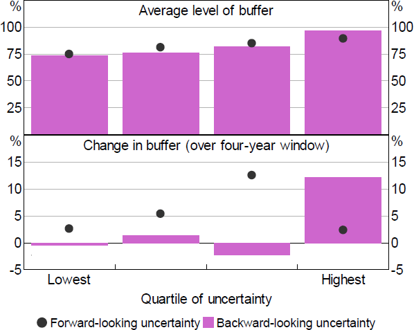
To examine the role of income uncertainty in explaining the trend in liquidity buffer over time, the income uncertainty indicators are split into quartiles based on the level of uncertainty.[14] The top (bottom) quartile includes the households facing the most (least) income risk (Figure 16). The HILDA Survey estimates generally indicate that liquidity buffers increased more between 2002 and 2018 for the households facing higher income risk. This is mostly true of the backward-looking indicator. This suggests that precautionary saving behaviour explains some of the increase in liquidity buffers amongst households with mortgage debt. However, the share of households facing higher income risk is not large enough to fully explain the rise in aggregate liquidity buffers, suggesting that other forces are at play too.
| Forward-looking indicator (working mortgagor households) |
Backward-looking indicator (all mortgagor households) |
|
|---|---|---|
| Income uncertainty | 0.13* (1.89) |
0.25*** (3.46) |
| Disposable income (log level) | 0.06 (1.27) |
0.04 (0.92) |
| Housing price-to-income ratio | 0.03*** (2.84) |
0.02*** (2.67) |
| Fixed effects | No | No |
| R squared | 4.7 | 4.5 |
| Households | 3,708 | 3,958 |
| Observations | 7,170 | 7,704 |
|
Notes: *, ** and *** denote statistical significance at the 10, 5 and 1 per cent levels, respectively; standard errors are clustered by household with t-statistics in parentheses; the regressions are also bootstrapped to address the generated regressor for the backward-looking uncertainty indicator; coefficient estimates for the constant and dummies for loan age, age of household head and survey year are omitted Sources: Authors' calculations; HILDA Survey Release 19.0 |
||

Notes: Buffer measured as the ratio of household liquid assets to disposable income; liquid assets include the value of cash, deposits, equities, bonds, trusts and estimated redraw balances
Sources: Authors' calculations; HILDA Survey Release 19.0
5.3 The housing equity withdrawal and refinancing channels
There was considerable product innovation in the Australian mortgage market through the late 1990s and the first half of the 2000s (Debelle 2010). Lenders introduced products such as home equity withdrawal loans and reverse mortgages, which allows households to borrow against the equity they have built up in their homes. Lenders also introduced interest-only loans and shared equity loans, which made it easier for households, particularly first home buyers, to purchase homes.
Since that time, housing equity withdrawal (HEW) has become relatively commonplace in Australia, with close to one in ten borrowers withdrawing equity from their home in any given year, according to estimates from the HILDA Survey. A 2006 survey of home owners also indicated that more than half of the equity withdrawn was used for asset accumulation, with deposits accounting for around one-third of all withdrawn funds (Schwartz et al 2006). This is consistent with households rebalancing their portfolios towards liquid assets in response to greater housing wealth.
To examine the effect of these mortgage products on household liquidity, we study the liquid asset accumulation of borrowers in the HILDA Survey. We can split borrowers into those that report either having a home equity loan or have refinanced since they took on a mortgage. If debt amortisation is associated with higher liquidity, we should observe a negative correlation between the growth rate of debt and liquid assets for a given borrower over time. But if the housing equity withdrawal/refinancing channel is important in practice, we should observe a weaker negative correlation between mortgage debt amortisation and liquid asset growth for households that extract equity or refinance. This is because mortgage debt and liquid assets simultaneously increase, at least temporarily, in these cases.
To test this hypothesis, we estimate the following panel regression:
where the dependent variable is the dollar change in liquid assets each ‘period’ and the explanatory variables include the dollar change in mortgage debt , a dummy for whether the borrower reports refinancing or withdrawing equity within the current period ( HEWit ) and an interaction between that dummy and the change in mortgage debt . We also include a set of control variables for borrower characteristics that could matter to the accumulation of liquidity such as age, income and the growth rate of housing prices, as well as lagged levels of both liquid assets and mortgage debt. Note that by taking differences in balance sheet positions over time we also implicitly control for borrower characteristics that do not vary over time but could matter to the level of household liquidity, such as risk preferences or financial literacy.
As the full balance sheet of households is only reported every four years in the HILDA Survey, a ‘period’ here refers to a four-year window. As such, a borrower is reported to have refinanced or withdrawn equity if they report doing so at any time within the past four years. As the effect of equity withdrawal or refinancing on liquid asset accumulation is likely to be temporary (and perhaps only captured within a year of refinancing) the estimation of the regression using four-year windows may attenuate the estimates and make it more difficult to identify such a channel.
The regression estimates indicate that each dollar of mortgage amortisation is associated with an increase of around 8 to 10 cents in liquid assets, on average (Table 2, first row). This is consistent with mortgage debt amortisation being associated with an increase in the value of liquid assets. More importantly, the debt amortisation effect is weaker for loans that have either been refinanced or have been used for HEW (Table 2, second row). This is consistent with the process of HEW or refinancing being associated with temporary increases in both debt and liquidity. This provides evidence that households rebalance their wealth portfolios in response to higher housing prices by building more liquidity through such channels.[15]
| OLS | |||
|---|---|---|---|
| No controls | With controls | With interactions and controls | |
| Change in mortgage debt | −0.08*** (−7.69) |
−0.10*** (−7.67) |
−0.12*** (−7.47) |
| HEW * Change in mortgage debt | 0.05* (1.94) |
||
| Change in household disposable income | 0.24*** (3.75) |
0.24*** (3.74) |
|
| Change in housing prices | 0.07*** (5.17) |
0.07*** (4.92) |
|
| Fixed effects | No | No | No |
| R squared | 0.7 | 3.9 | 4.0 |
| Observations | 12,222 | 12,222 | 12,222 |
|
Notes: *, ** and *** denote statistical significance at the 10, 5 and 1 per cent levels, respectively; standard errors are clustered by household with t-statistics in parentheses; coefficient estimates for the constant and dummies for HEW, loan age, age of household head and year are all omitted; the sample period is every four years between 2002 and 2018 Sources: Authors' calculations; HILDA Survey Release 19.0 |
|||
Footnotes
We follow Simon and Stone (2017) to identify when households purchased their first home. [12]
The fitted values are estimated from a piecewise linear regression: Years since purchaseit * POSTit + Years since purchaseit * (1 – POSTit), where Years since purchaseit is the number of years since the home was purchased (which is negative for the years before purchase) and POSTit is a dummy variable which is equal to one if the year is after purchase and is zero otherwise. The underlying data on liquid assets is observed every four years in the survey. So, for example, a comparison of years 1 and 2 in the figure is a comparison of different households rather than the same household over time. This should be borne in mind when interpreting the trends in the figure. [13]
The distribution of the backward-looking uncertainty indicator is based on quartiles, while the distribution of the forward-looking indicator is based on terciles, with the bottom (low uncertainty) category including working households with an estimated subjective probability of zero job loss. [14]
An alternative way that home owners can extract home equity is by buying a home with less equity than their previous residence. We gauge the importance of this channel by studying the behaviour of liquidity buffers in the year of moving for moving home owners (treatment group) relative to moving renters (control group) within the same postcode. We find that home owners do increase their holdings of liquid assets during this period of moving, while the liquid asset holdings of renters remains relatively unchanged. This is again consistent with home owners choosing to rebalance their wealth portfolios in response to higher housing prices through a HEW channel. However, the effect appears to be concentrated amongst outright home owners. This channel therefore cannot explain the rise in liquidity buffers amongst households with mortgage debt. [15]