Research Discussion Paper – RDP 2024-04 Nowcasting Quarterly GDP Growth during the COVID-19 Crisis Using a Monthly Activity Indicator
1. Introduction
What is happening in the economy now? It is said that the future is uncertain, but so is the present. Policymakers operating in this environment need some way to understand what is happening now (i.e. current economic conditions). This need for timely information was most acute during the COVID-19 crisis when current conditions were rapidly evolving, requiring policymakers to make decisions under significant economic uncertainty. Policymakers are further hamstrung because the most comprehensive measure of economy activity, gross domestic product (GDP), is published with a substantial lag. Indeed, the full effect on economic activity of the first major lockdowns which occurred during June quarter 2020 were not realised until the release of National Accounts data in early September 2020; more than two months after the reference period.[1] This delay limits its value to policymakers as a measure of the current state of the economy. Additionally, GDP is often revised in subsequent quarters which further limits its usefulness to policymakers for assessing current conditions.
In response, more and more higher-frequency partial indicators have become available in recent times; however, they are often not as comprehensive in their scope and coverage as traditional measures of economic activity such as GDP. And while these partial indicators do help fill the information gap, the signal they provide is often noisy. Further, one indicator might be useful in one context but not in another. For example, the unemployment rate is considered a key metric of economic activity, but during the COVID-19 crisis the Australian Government introduced the ‘JobKeeper’ program to keep workers employed, thereby limiting the rise in the unemployment rate caused by lockdowns.[2] During this period, the underemployment rate was considered to provide a more accurate signal. Given this, it is not clear how policymakers should choose which indicator to focus on, and if there are multiple indicators available, how much weight they should give to each one. The answers to these decisions are subjective and will typically vary with time and across policymaker.
What is required is a method of combining the available partial indicators in a systematic manner to smooth out the noise and reveal the underlying signal. The most common tool for achieving this is via dynamic factor models (DFMs). DFMs are a dimension reduction technique that can summarise the common variation across a panel of time series data.[3] In Australia, initial work exploring the usefulness of factor models for monitoring economic activity was undertaken by Gillitzer, Kearns and Richards (2005). They produced two coincident indicators, one summarising quarterly data and another summarising monthly data. Both indicators were estimated using the non-parametric methods developed by Stock and Watson (2002) and Forni et al (2000).[4] This was followed by Sheen, Trück and Wang (2015), who introduced a daily business cycle indicator based on the work of Aruoba et al (2009). Their method uses a parametric estimation technique involving a state-space model estimated using the Kalman filter.
Besides being a successful tool for monitoring activity, another important use of DFMs is for prediction (Stock and Watson 2002), especially in relation to producing nowcasts.[5] A significant amount of research effort has been devoted to this topic since the early works of Nunes (2005) and Giannone, Reichlin and Small (2008) (see Bańbura et al (2013)). However, there has been considerably less work done in Australia. For prediction, Gillitzer and Kearns (2007) had success, showing factor-based forecasts for key macroeconomic series can outperform standard time series benchmarks.[6] The benefits of DFMs are less clear when focusing explicitly on nowcasting in Australia (Australian Treasury 2018; Panagiotelis et al 2019). Using different estimation techniques both suggest the sample mean is a difficult benchmark model to beat in relation to nowcasting quarterly GDP growth.[7] But, while both works consider higher frequency data (monthly and higher), neither exploit this information in their nowcasting investigation. Instead, both convert all series in their respective datasets to a quarterly frequency before producing a nowcast.[8],[9] This is a problem because it represents a loss of information. Further, there is extensive research highlighting the significant improvement in prediction accuracy that comes from working with mixed frequency data.[10]
Our work bridges the gap that exists in the literature between employing factor models for monitoring and for nowcasting in Australia. Both issues are interrelated and are equally important for policymakers, so it is sensible to develop a framework that can achieve both objectives at once. In doing so, we build on previous work in Australia by incorporating more recent developments in factor modelling and nowcasting. We start by developing a monthly activity indicator (MAI) for Australia. The MAI aims to provide policymakers with a more immediate snapshot of prevailing economic conditions. We achieve this by using a ‘true’ DFM to summarise the information content from a dataset of 30 monthly targeted predictors selected for their ability to explain movements in first-release quarterly GDP growth.[11] This is an important advance compared to previous studies as it links the variable of interest to the estimation of the DFM and has been shown to improve factor estimation and predictive ability (Bai and Ng 2008; Bulligan, Marcellino and Venditti 2015). We also extend the targeted predictor hard thresholding pre-selection step developed by Bai and Ng (2008) when estimating factor models to the mixed frequency setting. Further, the methodology we use to estimate the MAI allows us to use an unbalanced dataset which therefore means we can consider a broader collection of series over a longer time period than the competing indicators produced by Gillitzer et al (2005) and Sheen et al (2015).
Unlike previous nowcasting studies in Australia (e.g. Australian Treasury 2018; Panagiotelis et al 2019), which have focused exclusively on quarterly frequency data, we undertake the first investigation of nowcasting in Australia using a mixed frequency modelling framework. We exploit the MAI's high-frequency information content within a factor augmented unrestricted MIDAS (MIxed Data Sampling) model (FA-U-MIDAS).[12] We assess the model's ability to nowcast first-release quarterly GDP growth using a recursive out-of-sample evaluation exercise covering a 34-year period (1988:Q2–2022:Q2), longer than previous works including Gillitzer and Kearns (2007), Australian Treasury (2018), and Panagiotelis et al (2019). Additionally, since we use monthly data, we can generate four nowcasts for each quarterly GDP growth observation as new monthly data becomes available across the quarter. Finally, as in previous evaluations, we use the standard benchmark forecasting models of the sample mean and an AR(1) process for comparison.
Our results show that incorporating monthly information provides more accurate predictions compared to the benchmark models based on smaller estimated root mean squared error. The improvement over the benchmark models (sample mean and AR(1) models) is also found to be statistically significant as well.[13] Crucially, predictive accuracy of the models with monthly data is largest during the COVID-19 crisis compared to the benchmark models relying solely on quarterly data, highlighting the benefit to policymakers from having timely information. Our results also support previous findings which suggest that model predictive performance can change depending on the state of the economy (see Chauvet and Potter (2013), Siliverstovs (2020) and Jardet and Meunier (2022)).
We begin by describing in detail the methods we follow to construct the MAI in Section 2. In Section 3 we discuss how we use the MAI to predict quarterly GDP growth as well as the steps we follow to implement the out-of-sample evaluation exercise before concluding in Section 4. Some additional results are provided in the appendices.
2. Monitoring Activity Using a Combination of Targeted Monthly Indicators
To construct the MAI, we apply a DFM to a monthly dataset. The dataset will be comprised of series which show a statistically significant relationship with quarterly GDP growth since this is our variable of ultimate interest. We first discuss the monthly dataset and how we select the series it contains before describing the DFM method and estimation results.
2.1 Monthly activity dataset
The choice of dataset to use when estimating a DFM is an important part of the process that is often underappreciated. There no single agreed upon way to do this in the literature. Indeed, different datasets can result in different factor estimates even when using the same estimation technique (Bai and Ng 2008). Given this, there is a tendency for researchers to select as many series as possible in the attempt to capture all available information. However, having too many series can be problematic for factor estimation as well; especially if many of the series in the dataset are ‘noisy’ (Boivin and Ng 2006).[14]
Relatedly, other methods for creating datasets from pre-selected series have been proposed to generate more accurate forecasts with factor-augmented regressions. Unlike those proposed by Boivin and Ng (2006), these methods recommend estimating a factor model using a dataset comprised of only those series shown to have predictive power for a ‘target’ variable of interest. Importantly, these so-called ‘targeted predictors’ explicitly take account of the object of interest which other methods do not. Two prominent strategies include ‘hard’ and ‘soft’ thresholding to determine which variables the factors are to be extracted from (Bai and Ng 2008). Under hard thresholding, the predictors are ranked based on a pre-test procedure and those that fail to meet some criteria are discarded from the dataset. Under soft thresholding, a portion of top ranked predictors are kept, where the ordering of the predictors depends on the soft thresholding rule used. Bai and Ng (2008) show that factors extracted from a dataset of targeted predictors can result in superior forecasting performance.[15]
To begin, we compile an ‘extended’ dataset that includes 53 monthly partial indicators covering various aspects of the Australian economy. Following Bańbura and Rünstler (2007) we group these series into three main categories: ‘hard’ (30 per cent; includes series covering key measures of activity such as the labour market); ‘soft’ (36 per cent; includes survey measures which tend to be more timely than hard series); and ‘financial’ (34 per cent; includes series such as interest rates, equity prices and commodity prices). When available, we include both aggregate and disaggregate measures in the dataset (i.e. total credit as well as its sub-components). Some researchers argue against this practice; however, the method we use to estimate the DFM is robust to including aggregate and disaggregate series.[16] The dataset covers the sample period 1978:M2 to 2022:M9 and was influenced by the number of series available in the early part of the sample.[17] However, several series in the dataset have later starting and earlier ending periods due to being relatively new, so the resulting dataset is ‘unbalanced’ or ‘ragged edge’.
Before using the dataset, we transform all series to be stationary and standardise them to have zero mean and unit variance as is common in the factor modelling literature. Series are made stationary by taking logs and/or first differences as appropriate (see Table A1 for details). When doing the standardisation, rather than use the full sample mean, we instead follow Kamber, Morley and Wong (2018) and implement ‘dynamic demeaning’ for each series using a rolling 20-year backward-looking estimate of the sample mean as a way of controlling for potential structural breaks in the central tendency of each series over the sample period the dataset covers. The decision to use a 20-year window (instead of a 10-year window as in Kamber et al (2018)) is because until the COVID-19-induced recession in 2020, the length of the business cycle in Australia was arguably longer than elsewhere.[18]
Since our main goal is to produce a monthly activity indicator for monitoring the economy at a higher frequency than is currently possible and to predict quarterly GDP growth in the near term, we will follow Bai and Ng (2008) and implement a pre-selection strategy to our extended dataset to remove any uninformative predictors in relation to quarterly GDP growth. Because our dataset is unbalanced, we will use their hard thresholding strategy. This involves running a series of separate regressions of the target on a single predictor. Each regression includes a set of controls comprised of an intercept and lags of the target variable which are the same for all regressions. The predictors are then ranked in descending order by the magnitude of the coefficient t-statistic on each predictor. Any predictor with a test statistic below some specified threshold significance level is discarded.[19],[20]
The method we use to estimate the DFM is robust to model misspecification. Hence, one could argue there is no need to apply any pre-selection to the dataset since the model will assign the right weight to each series (see Bańbura et al (2013)). However, factors extracted from the extended dataset will, by construction, be a linear combination of all series in the dataset. Some of these series might not be very informative about quarterly GDP growth but will still have some effect on the model outputs even if small. That is, no series is likely to be assigned a zero weighting. Therefore, it makes sense to only focus on a subset of series found to be informative about the quarterly growth in GDP.[21]
Instead of using the current release version of GDP, which is a combination of first release, revised and fully revised data (Stone and Wardrop 2002), we follow Koenig, Dolmas and Piger (2003)'s recommendation and use the first-release version of GDP (Lee et al 2012). We extend Bai and Ng (2008)'s hard-thresholding algorithm (which only considers variables at a quarterly frequency) to a mixed frequency setting. This is because our target variable is quarterly while our predictors are monthly. In this situation, it is typical to perform some type of temporal aggregation such as taking the quarter average (i.e. each quarterly observation is the average of the three monthly observations in each quarter). However, this could result in a potential loss of information. Instead, each monthly series is converted to a quarterly series by stacking the first, second and third months in each quarter as three separate quarterly series.[22]
Because we have three predictors (i.e. one series each for the first, second and third months of the quarter) instead of only one as in Bai and Ng (2008) and Bulligan et al (2015), we cannot implement the same t-statistic to test for significance and rank series as they both do. Instead, we test for the joint (linear) significance for all three series at once using a Wald statistic calculated using a HAC robust covariance matrix. As controls we include an intercept and, as our sample covers the COVID-19 crisis period, a set of seven indicator variables for the periods 2020:Q2 to 2021:Q2 and 2021:Q4.[23] The indicator variables were included to account for the COVID-19 crisis so as not to affect the test results and series ranking.[24] When running each regression, we adjust the dependent variable's sample length to match the sample length of each predictor which varies by series. Because our extended dataset is already relatively small by international standards, we use a less restrictive significance level of 10 per cent to gauge significance.[25] While this is higher than the standard 5 per cent, it helps ensure we have a reasonable sized subset of the extended dataset.
The outcome from the hard thresholding procedure is a dataset of 30 variables from the original 53-variable extended dataset.[26] Of the three categories, ‘soft’ is the dominant one with 13 series (43 per cent); followed by ‘financial’ with 9 (30 per cent) and ‘hard’ with 8 (27 per cent). Figure A1 shows the 30 series by category and ranked by Wald statistic along with the threshold critical value (dashed line). The number of series in the targeted predictor dataset is comparable to the minimum suggested by Bai and Ng (2008) and is slightly larger than the 24 series used in the empirical application by Bańbura et al (2013) and slightly smaller than the 37 series used by Australian Treasury (2018). Further, Panagiotelis et al (2019) mention they find no benefit from considering an information set bigger than 20 to 40 variables when forecasting Australian macroeconomic time series such as quarterly GDP growth.[27]
2.2 Constructing the monthly activity indicator using a dynamic factor model
DFMs are a popular statistical model for summarising the common (linear) variation contained in a panel of time series data and prediction. A key issue of all these previous works is that they not true DFMs as per Bai and Wang (2015). Instead, we estimate the MAI using the general form of the DFM defined as:
where yt is a N × 1 vector of weakly stationary targeted predictors, ft is a q × 1 vector of the dynamic factors, and is the dynamic factor loadings for ft–i with i = 0, 1,...,s and t = 1,...,T. Together, the factors and loadings provide a measure of the common variation shared across series in the dataset. The dynamic factors are modelled as a VAR(p) process with a q × q matrix of autoregressive coefficients (with all roots outside the unit circle). The number of dynamic factors is q (the dimension of ft).
The covariance matrix of the idiosyncratic component is given by R with dimension N × N and is restricted to be a diagonal matrix. In the state equation, the covariance matrix of corresponds to the q × q matrix Q . We assume that (i.e. the two noise processes are independent). This specification of the DFM has two different sources of dynamics. First, there are s lagged factors representing a dynamic relationship between the observable series yt and the factors ft. Second, the dynamics of the factors are assumed to be captured by a VAR(p) process.[28] Bai and Wang (2015) argue that it is the first source of dynamics that makes this specification a true dynamic factor model because it is these dynamics that make the biggest distinction between dynamic and static factor analysis.[29]
We estimate the DFM by quasi-maximum likelihood (QMLE).[30] Estimation is conducted via the expectation-maximisation (EM) algorithm and consists of two parts. First, we estimate the factors given the data by running the Kalman filter and Rauch-Tung-Striebel (RTS) smoother recursions (the ‘E-step’). Second, we use the estimated factors from the previous step to compute the model parameters by maximising the expected log-likelihood by regression (the ‘M-step’). This requires us to re-cast Equation (1) into its state-space representation given as:
The measurement equation takes the form of a static factor model (Stock and Watson 2002) with r = q (s + 1) static factors. Let k = max(p, s + 1), then Ft is a qk × 1 vector of the dynamic factors and their lags, is a N × qk matrix of dynamic factor loadings, is a qk × qk companion matrix and G is a qk × q selector matrix. The advantage of using the state-space modelling framework is that it can easily and efficiently accommodate unbalanced datasets. See Hartigan and Wright (2023) for more details on the parameters and estimation procedure we use.
2.2.1 Determining the optimal DFM specification
Before we can estimate the DFM we first need to specify four important features. These are: i) the number of dynamic factors ( q ), ii) the number of dynamic loadings ( s ), iii) the lag order for the factor VAR in the state equation ( p ), and iv) the ‘named factor’ necessary for identification.
We use the information criterion developed by Hallin and Liška (2007) to determine the number of dynamic factors. This suggests there is only one common dynamic factor in the targeted predictor dataset (see Figure A4).[31] To set the number of dynamic factor loadings, we follow the strategy implemented in Luciani (2020). This exploits the fact that a dynamic factor model with q factors can be re-cast as a static factor model with r = q (s + 1) static factors as previously mentioned. Practically, we take a balanced subset of the targeted predictor dataset and compare the proportion of explained variation from the first r eigenvalues from the contemporaneous covariance matrix to the proportion of variation from the first q dynamic eigenvalues from the spectral density matrix averaged over a grid of frequencies (see Forni et al (2000) and Brillinger (1981) for more details). The aim here is to find where there is close agreement between these two measures. Examining Table 1 indicates that one dynamic eigenvalue (i.e. q = 1) explains approximately the same amount of variation as three static eigenvalues (i.e. r = 3) and hence suggests s ≈ 2. Further, Luciani (2020) argues that with s = 2 each series in the targeted predictor dataset is capable of loading on the dynamic factor in a time window of three months. This is interesting as this window corresponds to one quarter.
| Eigenvalue | |||||||||||
|---|---|---|---|---|---|---|---|---|---|---|---|
| (1) | (2) | (3) | (4) | (5) | (6) | (7) | (8) | (9) | (10) | ||
| Dynamic ( q ) | 60.0 | 72.5 | 80.8 | 86.8 | 90.6 | 93.6 | 95.9 | 97.6 | 98.9 | 100.0 | |
| Static ( r ) | 38.0 | 55.1 | 62.3 | 67.8 | 72.0 | 76.1 | 79.6 | 82.5 | 85.0 | 87.1 | |
| Notes: Dynamic eigenvalues estimated from the spectral density matrix of a balanced subset of the targeted predictor dataset averaged over a grid of frequencies from to ; static eigenvalues estimated from the contemporaneous correlation matrix of a balanced subset of the targeted predictor dataset. Bold values denote optimal number of factors. | |||||||||||
We can check whether Boivin and Ng (2006)'s suggestion that reducing the sample size can ‘sharpen the factor structure’ by comparing the amount of explained variation from the extended dataset and targeted predictor dataset. Focusing only on the first dynamic eigenvalue, the amount of variation explained in a balanced subset of the extended dataset is about 52 per cent (not shown), lower than the per cent of explained variation in the pre-screened dataset (Table 1). Hence, removing any series considered uninformative in relation to explaining movements in quarterly GDP growth has increased the signal-to-noise ratio of the common dynamic factor.
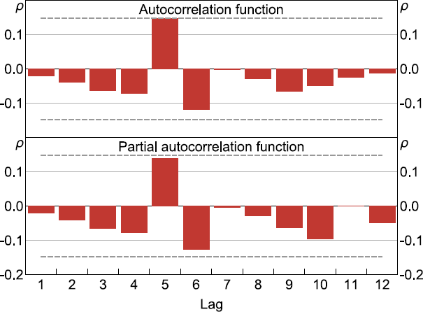
With only one common factor, the dynamics of the factor follow an AR process instead of a VAR process. To determine the lag order of the AR process we set this to one (i.e. p = 1) based on the AIC.
The final task needed before estimation can take place is identification. To identify the DFM we impose the ‘named factor’ normalisation (Stock and Watson 2016), which associates a factor with a specific variable.[32] In deciding which targeted predictor to make the named factor we put ‘WMI consumer sentiment’ as the first series because this series has the highest Wald statistic of all the 30 targeted predictors (see Figure Al).
2.2.2 Estimation results
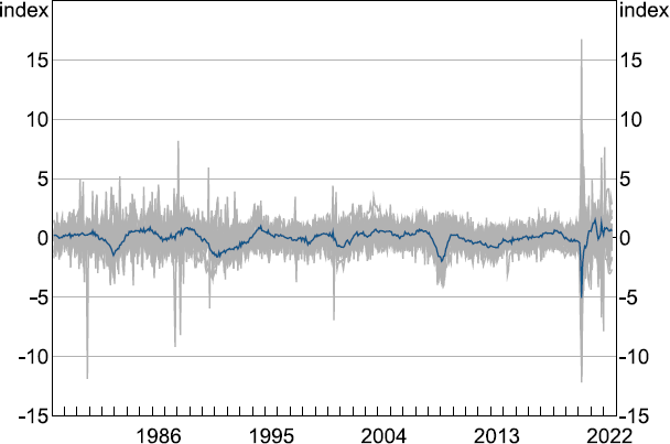
Figure 1 presents the (optimal) filtered estimate of the MAI for the sample period: 1978:M2 to 2022:M9.[33] The MAI reveals three periods of relatively weak activity that correspond with previous recessions in Australia, with the most recent being from the COVID-19 crisis (i.e. 1982, 1989-1991 and 2020). Indeed, the decline in the level of the MAI during this period is the largest ever observed in the series. Although the duration was much shorter than compared to the other two time periods and is focused predominately in June 2020.
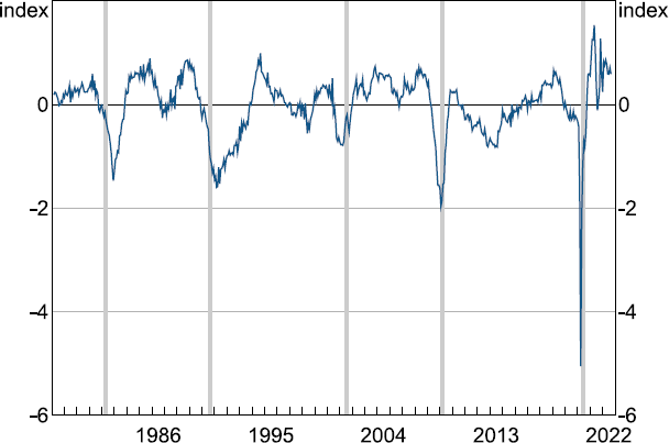
Note: Shaded bars are Sahm rule recession onset dates for Australia, defined as a ¾ percentage point increase in the three-month moving average of the unemployment rate relative to its minimum in the previous twelve months.
The MAI also shows activity was noticeably weak in two other periods which have not previously been considered as recessions as per the technical definition of a recession. The first period, 2001, is linked to the aftereffects of the introduction of the GST which caused a significant amount of activity to be brought forward. The second period, 2008, corresponds with the global financial crisis (GFC). However, both periods together with the three previously acknowledged recessions are detected by the so called ‘Sahm rule’ (Sahm 2019). This is an algorithm for detecting the onset of recessions based on monthly movements in unemployment and has correctly detected every recession in the United States since the 1970s as identified by the NBER, with no false positives.[34] We adjust the Sahm rule for Australia and consider a ¾ percentage point increase in the three-month moving average of the first-release unemployment rate relative to its minimum during the previous twelve months to be more appropriate. With no widely recognised recession timing for Australia equivalent to the NBER Business Cycle Dating Committee for the United States the Sahm rule serves as a useful proxy (see He and Rosewall (2020)). Figure 1 also shows that downturns in the MAI appear to occur several months before detection by the Sahm Rule. In this sense, the MAI provides an important signalling device for policymakers related to probable downturns.
To understand movements in the MAI over time we need to quantify the contributions of individual series. This is something not directly possible to do via non-parametric techniques such as PCA. These contributions are not provided as part of the estimation procedure, but they can be obtained from the state-space representation of the model in Equation (2). First, we take the state equation part of the model and re-write this expression in terms of the updating equation from the Kalman filter:
where Kt is the Kalman Gain at time t and is of dimension r × N and the other parameters are as previously defined. Equation (3) says that the estimate of the common factor at time t is a linear combination of a prediction step (based on information at t–1) and an update step based on the error in the prediction weighted by the Kalman Gain. This second part gives us the contribution from each series to the factor at each time point (see also Sheen et al (2015)).
Next, let Dt denote a r × N matrix of series-specific contributions and using Equation (3) we can get an expression for the update step for each series:[35]
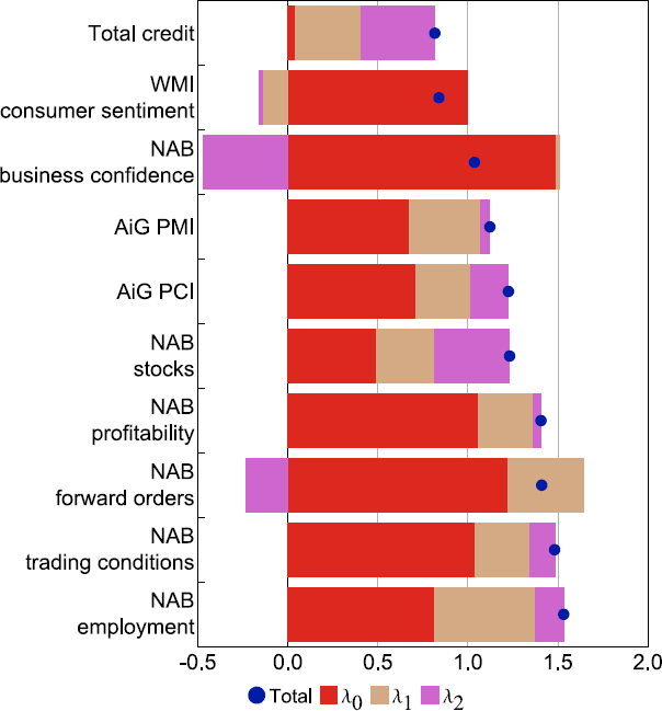
Equation (4) is related to Equation (3) by noting that where is a column vector of 1s with the number of elements specified by m. The first row of Dt for t = 1,...,T gives the individual series-specific contribution to the common dynamic factor ft as defined in Equation (1). Figure 2 plots the contributions to the Kalman filter estimate of the MAI aggregated by data category (i.e. hard, soft or financial) for the period January 2000 until July 2022 to allow for a more easy interpretation of recent history.
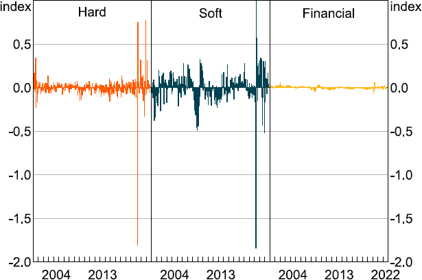
Note: Contribution to state update in Kalman filter recursions.
Figure 2 reveals the soft data category is the main contributor to updates in the MAI followed by hard and financial data. What is interesting about this observation is that the GFC was typically thought of as a financial crisis. However, the break down of the MAI by data category in Figure 2 reveals the previously discussed weakness in the MAI that occurred during the GFC in Australia was primarily due to a decline in soft data and these are mostly sentiment-based series.[36] Financial-based series only contributed a very small amount during that period.
This makes sense because during the GFC the economic environment was very uncertain and there was a lot of pessimism expressed by both consumers and businesses. However, fears of a serious recession turned out to be premature due to a combination of a very large fiscal response by the Australian Government, a very aggressive loosening of monetary policy by the RBA and a surge in demand for commodities from China. The steady rise observed in the MAI until early 2018 was also predominately caused by soft data. More recently, the dramatic movements observed in the MAI during the COVID-19 crisis period were due to contributions from both the hard and soft data categories, with the financial data category only making a relatively minor contribution.
This analysis reveals a potential issue that users of the MAI as a measure of activity need to consider. While soft data, such as surveys, do have the advantage of being very timely compared to hard data categories, they can also provide false signals (Aylmer and Gill 2003). Further, Roberts and Simon (2001) conclude that the information content that survey data, such as sentiment indicators, does provide is at best only a rough summary of prevailing economic conditions. However, they note that in some cases a linear combination of survey indicators (as is the case with a DFM) might not be a bad compromise.
As previously stated, the DFM we use to construct the MAI has been shown to be robust to misspecification including conditional heteroskedasticity and ‘fat tails’ (i.e. outliers) when the factors are extracted from many variables (see Doz et al (2012) and Bańbura et al (2013)). However, it is evident from Figure 1 that the COVID-19 crisis had a substantial effect unlike anything observed before on many of the series included in the targeted predictor dataset. Further, Maroz, Stock and Watson (2021) document how the COVID-19 crisis resulted in a temporarily large change in previously observed patterns of co-movement across a panel of US monthly time series data. While they use a different model than we do, it is still important to check the robustness of our model estimation.
The way we do this in our work is to compare two versions of the MAI constructed using parameters estimated from the full sample (including the COVID-19 crisis, labelled ‘FS’) and parameters estimated up to 2020:M2 (i.e. the pre-COVID-19 crisis, labelled ‘PC’). The results are illustrated in Figure 3 (upper panel) while the difference between the two MAI estimates is displayed in the lower panel. Visually, both MAI estimates look broadly similar. The main difference is that the PC estimate does not fall as dramatically during the worst of the COVID-19 crisis in June 2020. The sample standard deviation of the difference measure for the full sample is 0.15, while the sample standard deviation of the difference measure for the pre-COVID-19 sample is 0.11. The null hypothesis that the sample standard deviation of the full sample difference measure cannot be rejected at standard levels of significance.[37]
One reason for the smaller observed effect in our case compared to the findings of Maroz et al (2021) could be because our dataset does not display the same extreme movements during the COVID-19 crisis as their dataset. Indeed, they report one series having declined by more than 275 standard deviations. In our dataset, the largest decline was much smaller (see Figure A6). Further, given the relatively smaller decline observed in the MAI (PC) during the COVID-19 period, it is reasonable to argue that we need to include the COVID-19 period to ensure we correctly estimate its effect across series and the economy when we turn to nowcasting quarterly GDP growth in the next section.

Note: ‘FS’ refers to MAI based on parameters estimated using the full sample; ‘PC’ refers to MAI based on parameters estimated using a sample ending 2020:M2 (i.e. pre-COVID-19).
3. Predicting Quarterly GDP Growth Using the MAI
In this section we take the estimated MAI from the previous section and develop a framework for nowcasting quarterly growth in GDP. To achieve this goal, we will develop a regression model that relates the MAI to movements in quarterly GDP growth. This will require us to work with mixed frequency data.
3.1 Modelling mixed frequency data
When modelling time series of different frequencies, the typical thing to do is convert all time series to the lowest observed frequency using temporal aggregation. Usually this involves computing the average of the observations of the high-frequency variable that occur between samples of the low-frequency variable. For example, with monthly/quarterly data this could involve taking the average of the three months in the quarter or the last monthly observation in the quarter. The former was the approach adopted by previous studies in Australia including Gillitzer and Kearns (2007), Australian Treasury (2018), Panagiotelis et al (2019).[38] And while it is simple to implement, it discards potentially important information about the timing of movements in the high-frequency variable. Indeed, the reason we developed the MAI was so we could exploit the timely information it provides.
Instead, we will employ the MIDAS regression modelling framework (see Ghysels et al (2004) and Ghysels et al (2007)). MIDAS regression provides a flexible way to directly exploit all the information content of a higher-frequency explanatory variable to predict a lower-frequency dependent variable. It achieves this by using highly parsimonious distributed lag polynomials to prevent parameter proliferation that might otherwise occur.[39] MIDAS regression has been successfully used for predicting macroeconomic and financial variables. Of relevance to our work, Clements and Galvão (2008) show that using monthly information on the current quarter leads to significant improvements in forecasts based on coincident indicators.
An alternative approach that other researchers have used to handle mixed frequency data is to specify a state-space model and estimate it using the Kalman filter (e.g. Bok et al 2017).[40] However, in comparison with MIDAS models no clear ranking of forecast performance between the two methods was found (Bai, Ghysels and Wright 2013). Overall, Bai et al conclude that MIDAS and state-space models give similar forecasts.[41],[42]
The simple MIDAS model incorporating a single regressor is given by:
where and L1/m is a high-frequency lag operator such that with m indicating the higher sampling frequency of the explanatory variable (for example, m = 3 when x is monthly and y is quarterly). The intercept is specified by while the coefficient captures the overall effect of the high-frequency variable x on y and can be identified by normalising the function to sum to one. We assume the residuals, are an iid sequence with mean zero and constant variance. Finally, K is the maximum lag length for the included high-frequency regressor.
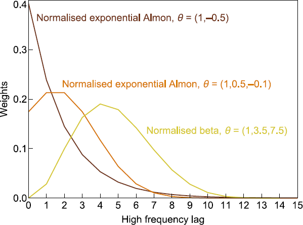
The method by which the MIDAS model achieves a parsimonious representation is via the lag coefficients in . This represents a set of weights as a function of a small dimensional vector of j parameters with . Two common functions used in empirical applications include the normalised exponential Almon lag function of Ghysels et al (2004) given as:
And the normalised beta function of Ghysels et al (2007) given as:
Note, Figure B1 illustrates examples of both polynomial weighting functions for different sets of parameters. Since both weighting functions are highly nonlinear, MIDAS models featuring either of them will need to be estimated by nonlinear least squares. An alternative specification proposed by Foroni et al (2015) is ‘unrestricted MIDAS’ (U-MIDAS). This method leaves the high-frequency lag coefficients unconstrained and can be estimated by OLS.[43] Foroni et al (2015) show that U-MIDAS is often preferable to standard (i.e. restricted) MIDAS (R-MIDAS) when modelling quarterly and monthly data because m is small. This reflects the fact that when the number of lags to model is relatively small, complications caused from having to estimate more parameters are reduced.[44] A U-MIDAS model with one explanatory variable is given as:
where and L1/m is defined as before. In any case, our x variable (i.e. the MAI) will be a latent common dynamic factor. MIDAS models incorporating factors are typically referred to as factor augmented MIDAS (FA-MIDAS) models and have been shown to perform well compared to more standard quarterly factor models in short-term forecasting of quarterly GDP growth in Germany (see Marcellino and Schumacher (2010)).[45] This finding is important for our work in two ways. It confirms the benefit to prediction from using mixed-frequency techniques and suggests that FA-MIDAS models can exploit time series information more efficiently than existing approaches.
Before we can move onto specifying a MIDAS model for nowcasting quarterly GDP growth using the MAI we need to decide on two aspects about the specification we intend to use. First, the functional constraints (if any) to implement and second, the optimal maximum lag order K. One way to address both issues is to use an information criterion to select the best model in terms of parameter restriction and the lag orders based on in-sample model fit.
Since the selected model will ultimately be used for nowcasting, we follow standard practice in the forecasting literature and use real-time data.[46],[47] For the dependent variable y we use first-release GDP from Lee et al (2012).[48] The main argument for this decision is that data revisions to GDP cause an additional issue when nowcasting. If we focus on current GDP, which is a combination of first release, partially revised and fully revised data, then we not only have to consider how to nowcast the first release of quarterly GDP growth but also how to predict future data revisions. Further, revisions to GDP can occur many quarters after the initial release. So, it is reasonable to assume analysts are more interested in the initial releases and concerned with the uncertainty related to nowcasting the first release than the uncertainty related to the revision process (Galvão and Lopresto 2020).
Unlike with GDP, there is no vintage targeted predictor dataset available for constructing a genuine real-time version of the MAI. However, as an alternative, we use the estimate of MAI produced by the Kalman filter for the reason previously discussed about it being more appropriate for prediction since it only incorporates information up to time t. Further, it is also conceptually similar to the definition of a real-time variable provided by Koenig et al (2003).[49]
We follow Foroni et al (2015) and use the BIC to evaluate a range of restricted and unrestricted MIDAS models. For the R-MIDAS models, we consider the normalised exponential Almon weighting function with j = 2 and j = 3 parameters. We also consider the normalised beta weighting function with j = 3 parameters. For all MIDAS model specifications, we specify four values for the maximum lag of the monthly explanatory variable (i.e. K ).[50] The results are presented in Table 2. The BIC strongly prefers the U-MIDAS specification with maximum lag K = 5, this is closely followed by the U-MIDAS model with maximum lag K = 6. Indeed, all U-MIDAS models are superior to the two R-MIDAS models except for when the maximum lag is two (K = 2). In this case, the R-MIDAS model using the normalised exponential Almon polynomial weighting function with two parameters (j = 2) is preferred.
In addition to comparing models based on the BIC, it is also possible to test the empirical adequacy of the polynomial weighting functions used with the R-MIDAS specifications under standard assumptions via a Wald-type test. The null hypothesis is that the functional restrictions are valid. Therefore, rejecting the null implies the functional restrictions are not supported by the data. By this metric, only one R-MIDAS model specification is consistent with the data, corresponding to the normalised exponential Almon polynomial weighting function with K = 2 and j = 2.
| Lag 0 : K |
Normalised exponential Almon | Normalised beta | U-MIDAS | ||||||||
|---|---|---|---|---|---|---|---|---|---|---|---|
| j=2 | j=3 | j=3 | |||||||||
| BIC | p-value | BIC | p-value | BIC | p-value | BIC | p-value | ||||
| 0:2 | 486.88 | 0.86 | 492.05 | 0.00 | 505.09 | 0.00 | 491.35 | na | |||
| 0:3 | 500.63 | 0.00 | 492.06 | 0.00 | 492.06 | 0.00 | 437.71 | na | |||
| 0:4 | 501.95 | 0.00 | 492.06 | 0.00 | 492.08 | 0.00 | 417.46 | na | |||
| 0:5 | 502.19 | 0.00 | 492.06 | 0.00 | 492.24 | 0.00 | 422.58 | na | |||
| Notes: The variable j is the number of parameters in the polynomial weighting function used in the MIDAS regression; the p-value is for the test of the null hypothesis of whether the restrictions on the MIDAS coefficients implied by the polynomial weighting function are supported by the data. Bold values denote best model. | |||||||||||
3.2 Out-of-sample prediction comparison
In this section we will assess the nowcasting performance of MIDAS models incorporating the MAI compared to standard benchmark models in a pseudo out-of-sample (OOS) comparison exercise. Based on the findings of the model evaluations presented in Table 2 we will only consider the FA-U-MIDAS specification for nowcasting quarterly GDP growth. However, instead of setting K = 5 as suggested by the BIC, we set K = 6. This choice is motivated by previous work (see Koening et al (2003) and Leboeuf and Morel (2014)) and because it covers the months most likely to affect quarterly GDP growth (i.e. three months of data covering the quarter for which we observe the last value of real GDP growth and the three months of data covering the first quarter to nowcast).[51]
We do not consider longer horizon predictions of quarterly GDP growth as in other studies. This is because predicting output growth over longer horizons is known to be much less reliable (e.g. Marcellino and Schumacher (2010) for FA-MIDAS models, Bańbura et al (2013) for factor models, and Chauvet and Potter (2013) for a systematic evaluation more generally). As such, the methods we develop here should only be thought of as short-term prediction devices.
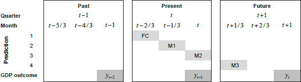
An important advantage of MIDAS regression over other methods used for handling mixed frequency data (i.e. temporal aggregation) is that it allows us to make predictions within periods. Further, each successive prediction will incorporate a new estimate of the MAI as more data becomes available in the quarter. For simplicity, we assume the following timing of data releases. Let yt denote the current quarter of quarterly GDP growth and yt+1 denote the next quarter of quarterly GDP growth. The first release of GDP for quarter t contains data up to quarter t – 1. Before data on GDP growth for t become available in quarter t +1, we will have four updates of the MAI. First estimate of the MAI incorporating monthly data up to t –1 in t –2/3 (i.e. first month of current quarter), second estimate of the MAI incorporating monthly data up to t –2/3 in t –1/3 (i.e. second month of current quarter), third estimate of the MAI incorporating monthly data up to t –1/ 3 in t (i.e. end of the current quarter). Finally, a fourth estimate of the MAI incorporating monthly data up to t in t +1/3 (i.e. first month of the next quarter). The timing of these monthly updates of the MAI allows us to produce four predictions of quarterly GDP growth in the current quarter which we label as i) forecast (FC), ii) nowcast in month 1 (M1), iii) nowcast in month 2 (M2), and iv) nowcast in month 3 (M3).[52] See Figure 4 for a visual summary.
Based on this, the general FA-U-MIDAS model we use in the OOS evaluation becomes:
where yt is first-release quarterly GDP growth, xt is the MAI and depending on the monthly flow of data during the quarter (i.e. corresponding to the four predictions: FC, M1, M2, M3, in that order). Hence, as new monthly estimates of the MAI are produced during the quarter, the specification of the FA-U-MIDAS model will change with an increasing number of regressors. For example, when i =3 (i.e. FC), the FA-U-MIDAS model for current quarterly GDP growth consists of an intercept and three months of data on the MAI from the previous quarter:
Alternatively, when i =0 , the model expands to include three additional months of data on the MAI from the current quarter (reflecting the full model):
Note, for ease of notation, we drop the superscript (m) from the x variable in both equations. Across the OOS evaluation period we will keep the FA-U-MIDAS model specification fixed to this general form.[53] Further, we will compare the four FA-U-MIDAS model specifications to two standard models used in previous OOS forecasting/nowcasting evaluation exercises. These include the sample mean and an AR(1) process (see Australian Treasury (2018) and Panagiotelis et al (2019) for the sample mean and Gillitzer and Kearns (2007) for the AR(1) process). The sample mean has been shown to be a formidable forecasting model for quarterly growth in GDP (Panagiotelis et al 2019) and will serve as our benchmark model in our comparisons. Additionally, we also consider a model based on a quarter average (QA) measure of the MIA as a crosscheck.[54] The QA model includes a temporal aggregated value of the MAI for the current quarter and another lagged value for the previous quarter, making it similar to M3.
To evaluate the performance of the various models, we carry out a recursive estimation and forecast/nowcasting exercise, where the full sample is split into estimation and evaluation sub-samples. The estimation sample initially covers the period 1978:Q2–1988:Q1 (i.e. R = 40 or 10 years, similar to Panagiotelis et al (2019)) and is expanded by one quarter at a time and the model parameters are re-estimated each time. The evaluation sample is between 1988:Q2 and 2022:Q2 (i.e. P =137 ). For each quarter in the evaluation sample, we want to compute a forecast and three nowcasts depending on the monthly information set. For example, for the initial evaluation quarter 1988:Q2, we want to compute a forecast using data up to 1988:Q1 (FC) and then a nowcast in 1988:M4 (M1), 1988:M5 (M2) and 1988:Q2 (M3). At this point we also compute the sample mean and AR(1) forecasts. The predictions from each model over the evaluation sample are presented in Figure 5.
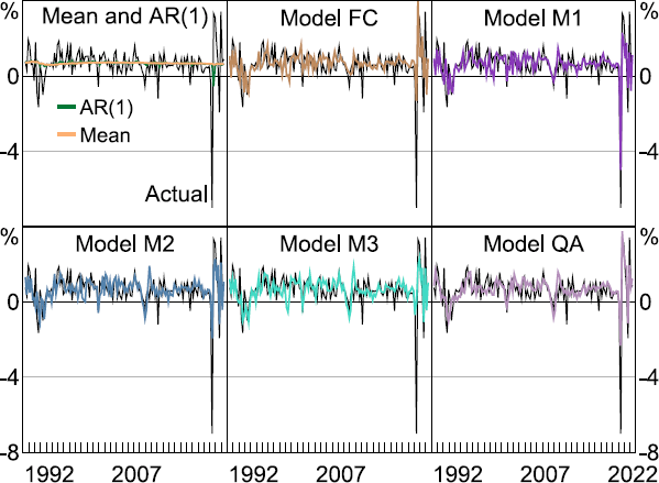
Note: GDP is first release.
Sources: ABS; Authors' calculations; Lee et al (2012).
The sample mean and AR(1) predictions are very similar given the lack of persistence in quarterly GDP growth, although the AR(1) model was slightly better at predicting the COVID-19 decline in 2020:Q2, albeit with a quarter lag. Since both models are estimated using quarterly data, neither were able to fully anticipate the significant fall and immediate rise that eventuated in 2020:Q2 and 2020:Q3. In contrast, the models incorporating monthly information performed much better. Predictions from each model are reasonably similar in the period before the COVID-19 crisis, but all models show noticeable differences in the period afterwards. For example, model M1 was most accurate in predicting the contraction in quarterly GDP growth in 2020:Q2, although it was still off by around 2 percentage points. Alternatively, model M3 was relatively less successful. This is surprising, since model M3 has two extra months of data on 2020:Q2 and previous research has shown that having more timely data usually improves forecast accuracy.[55] One explanation could be that model M3 has two additional parameters to estimate compared to model M1 and increased estimation uncertainty could be affecting the model's accuracy.
In relation to predicting the large subsequent upswing in quarterly GDP growth in 2020:Q3, more success was achieved by models FC and QA. This is also surprising since both models contain less information on the quarter compared to the three ‘M’ models. However, both models have less parameters to estimate compared to the other models (FC with three and QA with only two) and therefore could be more precisely estimated, improving the accuracy of both models.
We assess point forecast/nowcast accuracy of each model considered using standard root mean squared error (RMSE) defined as:
where is the forecast/nowcast produced by one of the models and P is the number of predictions being assessed. We compare RMSEs over three different horizons: the past three years, the past ten years, and the full evaluation sample period. We do this comparison for the full sample which includes the COVID-19 period as well as a sample that ends in 2019:Q4, excluding the effects of the COVID-19 crisis as a robustness check. The results are presented in Table 3 which provides both the raw RMSEs for each model computed using Equation (12) as well as the RMSE for each model relative to the sample mean model. A relative RMSE greater than one implies the model's predictions are less accurate compared to the benchmark model while a relative RMSE less than one implies the model's predictions are more accurate than the benchmark model.[56]
For the full sample period, model M1 outperforms all other models across each of the three horizons. In relative terms, model M1's RMSEs are over half of those of the sample mean model across the past three-year and ten-year periods and just under three-quarters of the benchmark model for the full sample. The QA model was the only other model that achieved a similar level of performance for the full sample horizon. As previously discussed in relation to Figure 5, this result is primarily because of how well model M1 predicted the significant decline in quarterly GDP growth that occurred in 2020:Q2. This is supported by comparing the model RMSEs in the pre-COVID-19 period. Here, there is no one model that outperforms the others in all periods as was the case when the COVID-19 period was included. Further, all model RMSEs are notably lower and much closer together as well. The models incorporating monthly information are not as dominant either. Indeed, the three ‘M’ models are outperformed by the sample mean model in both the shorter three-year and longer full sample horizons. In contrast, the QA model does narrowly outperform the benchmark model across all three horizons, suggesting that there is always some benefit to using timely information to make predictions. However, it also suggests that there might exist a trade-off between model size and accuracy, especially when making predictions during relatively ‘normal’ periods.
| Sample mean | AR(1) | FC | M1 | M2 | M3 | QA | |
|---|---|---|---|---|---|---|---|
| Full sample | |||||||
| Root mean squared error | |||||||
| Past three years | 2.72 | 2.83 | 2.11 | 1.24 | 1.72 | 2.23 | 1.49 |
| Past ten years | 1.52 | 1.58 | 1.19 | 0.74 | 1.00 | 1.26 | 0.87 |
| All | 0.98 | 1.01 | 0.87 | 0.70 | 0.78 | 0.88 | 0.70 |
| Relative root mean squared error | |||||||
| Past three years | na | 1.04 | 0.77 | 0.45 | 0.63 | 0.82 | 0.55 |
| Past ten years | na | 1.04 | 0.79 | 0.49 | 0.65 | 0.83 | 0.57 |
| All | na | 1.03 | 0.89 | 0.71 | 0.79 | 0.89 | 0.71 |
| Pre-COVID-19 sample | |||||||
| Root mean squared error | |||||||
| Past three years | 0.30 | 0.30 | 0.35 | 0.34 | 0.33 | 0.36 | 0.29 |
| Past ten years | 0.46 | 0.47 | 0.45 | 0.43 | 0.45 | 0.46 | 0.45 |
| All | 0.59 | 0.59 | 0.64 | 0.62 | 0.61 | 0.60 | 0.56 |
| Relative root mean squared error | |||||||
| Past three years | na | 1.00 | 1.18 | 1.15 | 1.10 | 1.21 | 0.98 |
| Past ten years | na | 1.03 | 0.98 | 0.94 | 0.97 | 1.01 | 0.97 |
| All | na | 1.00 | 1.09 | 1.06 | 1.05 | 1.03 | 0.96 |
| Notes: Relative to sample mean model. Full sample: 1988:Q2–2022:Q2; pre-COVID-19 sample: 1988:Q2–2019:Q4. Bold values denote best model(s) for each horizon. | |||||||
When comparing our results to those of previous studies related to forecasting/nowcasting quarterly GDP growth, it is only fair to focus exclusively on our pre-COVID-19 sample results. In this light, our results still show a clear benefit to using higher frequency (monthly) data for predicting lower frequency (quarterly) data. Both Australian Treasury (2018) and Panagiotelis et al (2019), who each focus on quarterly data, are unable to consistently outperform the sample mean benchmark model. However, Australian Treasury's model can beat the sample mean model once all data on the current quarter are available (the timing of which would be comparable to our M3 and QA models). In contrast, all FA-U-MIDAS models except M3 outperform the sample mean model on average over the last ten years, while the QA version shows outperformance across this timeframe as well as over the last three years and full sample (1988:Q2–2019:Q4).
3.3 Evaluating model performance during the COVID-19 crisis
As shown in Table 3, the three-year horizon which covered the COVID-19 crisis shows substantial divergence in the accuracy of model predictions incorporating monthly and quarterly information. Most of this outcome can be attributed to one time point: June 2020 – the quarter that experienced the brunt of the initial government-mandated COVID-19 lockdowns and the subsequent disruption to economic activity that resulted. The prediction error generated for each model relative to the actual first-release quarterly GDP growth outcome for that period is presented in Figure 6. A value above one means the prediction error was larger than the actual GDP outcome, while a value less than one signifies the prediction error was smaller than the actual GDP outcome.
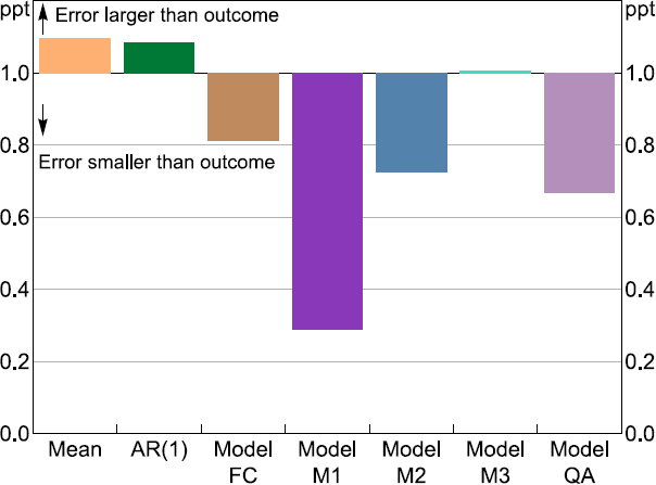
Note: Errors are relative to first-release quarterly GDP growth in 2020:Q2 (–7 per cent).
Figure 6 helps illustrate how incorporating high frequency (monthly) information greatly improved forecast/nowcast performance for most FA-U-MIDAS model predictions for this quarter, especially model M1 (which includes the month of April 2020 in its nowcast). Model M1 achieved a nowcast error equivalent to roughly one-quarter of the size of the eventual downturn that occurred in quarterly GDP growth (–7 per cent). What is crucial about this from a policymaker's perspective is the nowcast from model M1 was capable of being generated midway through the quarter in question – almost three months before the official figure on GDP would finally be published. Thereby giving policymakers a very timely reading on how the COVID-19 crisis was affecting activity.
Like with the prediction results, the errors for models M2 and M3, which include more timely information, are also both substantially larger than model M1. The performance of the QA model, which uses a temporal aggregated version of the MAI (i.e. three-month average), appears to strike a compromise between the three MIDAS models; suggesting there might be situations when it is beneficial to use temporal aggregated regressors in models, potentially in cases when the model might be otherwise over-parameterised. However, our key result that incorporating timely information can improve model prediction accuracy during downturns corresponds to previous work including Clements and Galvão (2009) (the US recession in 2001), Schorfheide and Song (2015) (the GFC impact on US economic activity in 2008) and Jardet and Meunier (2022) (the COVID-19 pandemic's effect on world GDP growth).
3.4 Assessing the predictive content of the MAI
The relative RMSE results in the previous section indicate that models incorporating monthly information generate more accurate predictions (and smaller errors) compared to the baseline sample mean model. However, to be definitive, it is important we compare model performance using a formal statistical test of equal predictive accuracy.
We cannot use the well-known Diebold-Mariano-West (DMW) t-type test for equal predictive accuracy since we are evaluating nested models (all models include an intercept). Instead, we follow the approaches of Clark and McCracken (2005) and Clements and Galvão (2009) and implement the bootstrap version of the MSE-F test of equal mean squared error (MSE) developed by McCracken (2007).[57] Let MSEi denote the MSE from model i for , then the test of equal predictive accuracy of the benchmark sample mean model (i.e. ) and the alternative model specifications considered are implemented using the following test statistic:
where P is the number of predictions being compared. A negative MSE-F implies that model i is less accurate compared to the sample mean model, whereas a positive MSE-F means the model i is more accurate. The bootstrap is used to compute the p-value for the MSE-F test and proceeds as follows. The sample mean model is estimated using the whole sample period of first-release quarterly GDP growth (as recommended by Clements and Galvão (2009)). From the model fit we take the estimated intercept and the variance of the residuals and simulate multiple time series trajectories from the sample mean model assuming Gaussianity.[58] For each one of the simulated time series trajectories, we apply the same recursive estimation and prediction steps we used with the actual data to calculate the MSE-F statistic for that replication. Note, the MAI is held fixed in each replication. We set the total number of replications in the bootstrap procedure to 1,000. The empirical p-value is calculated as the proportion of MSE-F statistics from the simulations that are larger than the MSE-F statistic computed using actual data. We implement the bootstrapped MSE-F test for the full sample including the COVID-19 period and a shorter sub-sample excluding the COVID-19 period as we did in relation to the RMSE comparisons in Table 3. The results are presented in Table 4.
| Sample mean | AR(1) | FC | M1 | M2 | M3 | QA | |
|---|---|---|---|---|---|---|---|
| Test statistic | |||||||
| Full sample | na | −7.12 | 36.43 | 132.87 | 80.47 | 34.86 | 135.34 |
| Pre-COVID-19 | na | −0.20 | −19.77 | −14.29 | −11.53 | −7.71 | 11.47 |
| Empirical p-value | |||||||
| Full sample | na | 1.00 | 0.00 | 0.00 | 0.00 | 0.00 | 0.00 |
| Pre-COVID-19 | na | 0.18 | 0.98 | 0.68 | 0.38 | 0.10 | 0.00 |
|
Notes: Benchmark model is the sample mean. Empirical p-value computed by bootstrap using 1,000 replications. Full sample is 1988:Q2–2022:Q2; pre-COVID-19 sample is 1988:Q2–2019:Q4. Bold values denote rejection of the null hypothesis. |
|||||||
The MSE-F test results confirm the findings in Table 3 and they also differ depending on whether the test is conducted on the full sample or the pre-COVID-19 sample. For the full sample we strongly reject the null hypothesis of equal predictive accuracy in relation to the sample mean model and all four FA-U-MIDAS models incorporating monthly information. However, the same is not true for the pre-COVID-19 sample, where the null is only rejected for model QA (although model M3 is borderline at the 10 per cent level).[59]
Overall, these results mirror those of Chauvet and Potter (2013) and Siliverstovs (2020) that relate to the accuracy of model predictions of quarterly GDP growth in the United States changing between expansions and recessions. In our case, the statistical evidence favouring models incorporating more timely information over simpler models based on quarterly information is mostly due to significant outperformance during the three-year period covering the COVID-19 crisis. In contrast, during more ‘normal’ times, the model predictions incorporating monthly information fail to meaningfully improve on those of the benchmark sample mean model. Considering Figure A3, this is not surprising. Australian quarterly GDP growth is serially uncorrelated. However, model QA which includes some information on the current quarter (albeit averaged), was able to consistently outperform the benchmark model in both sample periods. This suggests there might be a trade-off between incorporating more timely information and increasing model complexity.
4. Conclusion
We have made two important contributions to the factor monitoring and prediction literature related to Australia. First, we developed a monthly activity indicator with a very long history using a ‘supervised’ DFM model, with the explicit goal of providing policymakers with a timely snapshot on prevailing economic conditions. The time span covered by our MAI (45 years) is unmatched by previous work. Second, we have exploited the higher-frequency information imbedded in the MAI in a comprehensive nowcasting exercise covering a 35-year period and show statistically significant outperformance compared to standard benchmark models is possible. In this regard, our work is the first to apply a mixed frequency framework in a systematic manner.[60] Further, we show that outperformance was greatest during the COVID-19 period, emphasising the benefit of using monthly data.
One curiosity related to our results is unlike many other works in which the prediction of GDP growth becomes more accurate as more data on the quarter comes to hand, our results show the opposite and get less accurate. We speculate this is related to increased parameter uncertainty due to estimating progressively larger models. Further, the COVID-19 crisis caused very large outliers (otherwise known as ‘leverage points’ due to their effect on the estimated regression fit) which can have a substantial effect on parameter estimation.
Despite this, our results do have some encouraging news for policymakers. By using MIDAS-based models incorporating the (timely) MAI, we show it is possible to predict Australian quarterly GDP growth more accurately during crisis periods (such as during the COVID-19 crisis) – a situation when accuracy is needed most. This comes about because the higher-frequency information contained in the MAI means the MIDAS models are quicker to detect abrupt changes, thereby giving policymakers more time to react.
One potential limitation of our work is that we do not redo the pre-selection step to determine the targeted predictor dataset at each time point in the out-of-sample prediction evaluation exercise. Instead, the ranking is done only once and using the full sample. This could bring some issues with our results; however, we are restricted by the unbalanced nature of our dataset which starts with only 17 series and is not as large as in other studies which have also mostly considered balanced datasets. But since we are not seeking to compare predictive accuracy of factor(s) extracted from a targeted predictor dataset to non-targeted predictor datasets this is probably less of a concern. Nonetheless, in future iterations, the targeted predictor dataset should be reviewed and updated as required to ensure it continues to contain only series that are informative about quarterly GDP growth.
In future work we intend to investigate three extensions: non-traditional data; sparsity; and nonlinearity. During the COVID-19 crisis greater use was made of non-traditional data such as mobility. We have not included any of these types of data in our extended dataset, although previous work suggests there might be merit for doing so (e.g. Choi and Varian (2012), who show internet searches can have predictive content). The challenge with some newer non-traditional datasets relates to their relatively short histories, making them harder to incorporate into analysis such as ours. In our work we used a two-step approach to identify the targeted predictor dataset and then extracted the factor afterwards. Recent work from Mosley, Chan and Gibberd (2024) suggests it might be possible to combine these two steps into one by incorporating sparsity using a form of regularisation into the estimation step. Lastly, the DFM is necessarily a linear model. Perhaps there are benefits to nowcasting from considering nonlinear specifications instead.
Appendix A: Additional Monthly Activity Indicator Details
A.1 Additional MAI dataset details
| No | Series | Source | Category | Start date | End date | Transformation code |
|---|---|---|---|---|---|---|
| 1 | Total employment | ABS | Hard | 1978:M2 | 2022:M9 | LD |
| 2 | Full-time employment | ABS | Hard | 1978:M2 | 2022:M9 | LD |
| 3 | Part-time employment | ABS | Hard | 1978:M2 | 2022:M9 | LD |
| 4 | Unemployment rate | ABS | Hard | 1978:M2 | 2022:M9 | FD |
| 5 | Underemployment rate | ABS | Hard | 1978:M2 | 2022:M9 | FD |
| 6 | Hours worked | ABS | Hard | 1978:M2 | 2022:M9 | LD |
| 7 | Job advertisements | DoE | Soft | 2006: M1 | 2022:M9 | LD |
| 8 | ANZ Job vacancies | ANZ | Soft | 1999:M7 | 2022:M9 | LD |
| 9 | NAB Business conditions | NAB | Soft | 1997:M3 | 2022:M9 | LV |
| 10 | NAB Profitability | NAB | Soft | 1997:M3 | 2022:M9 | LV |
| 11 | NAB Trading conditions | NAB | Soft | 1997:M3 | 2022:M9 | LV |
| 12 | NAB Employment | NAB | Soft | 1997:M3 | 2022:M9 | LV |
| 13 | NAB Forward orders | NAB | Soft | 1997:M3 | 2022:M9 | LV |
| 14 | NAB Stocks | NAB | Soft | 1997:M3 | 2022:M9 | LV |
| 15 | NAB Business confidence | NAB | Soft | 1997:M3 | 2022:M9 | LV |
| 16 | NAB Capacity utilisation | NAB | Soft | 1997:M3 | 2022:M9 | LV |
| 17 | AiG Performance of manufacturing index | Ai Group | Soft | 2001:M5 | 2022:M9 | LV |
| 18 | AiG Performance of services index | Ai Group | Soft | 2005:M9 | 2022:M9 | LV |
| 19 | AiG Performance of construction index | Ai Group | Soft | 2003:M2 | 2022:M9 | LV |
| 20 | New company registration rate | ASIC | Soft | 1978:M2 | 2022:M9 | LV |
| 21 | ANZ-Roy Morgan Consumer financial situation next year | ANZ-Roy Morgan | Soft | 2008:M10 | 2022:M9 | LV |
| 22 | ANZ-Roy Morgan Consumer confidence index | ANZ-Roy Morgan | Soft | 2008:M10 | 2022:M9 | LV |
| 23 | WMI Consumer family finances next 12 months | WBC-MI | Soft | 1978:M2 | 2022:M9 | LV |
| 24 | WMI Consumer sentiment index | WBC-MI | Soft | 1978:M2 | 2022:M9 | LV |
| 25 | Retail trade | ABS | Hard | 1982:M4 | 2022:M8 | LD |
| 26 | Sales of new motor vehicles | VFACTS | Hard | 1978:M2 | 2022:M7 | LD |
| 27 | Revenue passengers, international, inbound | DoT | Hard | 1985:M1 | 2022:M7 | LD |
| 28 | Goods and services credits | ABS | Hard | 1978:M2 | 2022:M8 | LD |
| 29 | Goods and services debits | ABS | Hard | 1978:M2 | 2022:M8 | LD |
| 30 | Building approvals – residential, private | ABS | Hard | 1978:M2 | 2022:M8 | LD |
| 31 | Building approvals – housing, total | ABS | Hard | 1978:M2 | 2022:M8 | LD |
| 32 | Building approvals – other dwellings, total | ABS | Hard | 1978:M2 | 2022:M8 | LD |
| 33 | Building approvals – alterations and additions, total | ABS | Hard | 1978:M2 | 2022:M8 | LD |
| 34 | Building approvals – non-residential, total | ABS | Hard | 1978:M2 | 2022:M8 | LD |
| 35 | Auction clearance rate | CoreLogic | Soft | 2008:M5 | 2022:M9 | LV |
| 36 | Credit – total | RBA | Financial | 1978:M2 | 2022:M8 | LD |
| 37 | Credit – housing | RBA | Financial | 1978:M2 | 2022:M8 | LD |
| 38 | Credit – other personal | RBA | Financial | 1978:M2 | 2022:M8 | LD |
| 39 | Credit – business | RBA | Financial | 1978:M2 | 2022:M8 | LD |
| 40 | 3-month bank accepted bills/negotiable certificates of deposit | RBA | Financial | 1978:M2 | 2022:M9 | FD |
| 41 | Yields on Australian government bonds – 3-years maturity | RBA | Financial | 1992:M6 | 2022:M9 | FD |
| 42 | Yields on Australian government bonds – 5-years maturity | RBA | Financial | 1978:M2 | 2022:M9 | FD |
| 43 | Yields on Australian government bonds – 10-years maturity | RBA | Financial | 1978:M2 | 2022:M9 | FD |
| 44 | Yield spread, AGS 3-years less 3-month bank bill | RBA | Financial | 1992:M6 | 2022:M9 | LV |
| 45 | Yield spread, AGS 5-years less 3-month bank bill | RBA | Financial | 1978:M2 | 2022:M9 | LV |
| 46 | Yield spread, AGS 10-years less 3-month bank bill | RBA | Financial | 1978:M2 | 2022:M9 | LV |
| 47 | AUD trade-weighted index | RBA | Financial | 1978:M2 | 2022:M9 | LD |
| 48 | S&P/ASX 200 | Bloomberg | Financial | 1978:M2 | 2022:M9 | LD |
| 49 | Index of commodity prices | RBA | Financial | 1978:M2 | 2022:M9 | LD |
| 50 | Home value index | CoreLogic | Financial | 1980:M1 | 2022:M9 | LD |
| 51 | SWIFT customer-to-customer RTGS | RBA | Financial | 1998:M10 | 2022:M9 | LD |
| 52 | Credit card payments | RBA | Financial | 1985:M1 | 2022:M8 | LD |
| 53 | Debit card payments | RBA | Financial | 1994:M5 | 2022:M8 | LD |
| Notes: ‘ABS’ is Australian Bureau of Statistics, ‘DoE’ is the Department of Employment, ‘DoT’ is the Department of Transport, ‘WBC-MI’ is Westpac and Melbourne Institute. ‘Transformation code’ indicates the method used to transform the data to be stationary if necessary, ‘FD’ indicates first difference, ‘LD’ indicates log difference and ‘LV’ indicates level. | ||||||
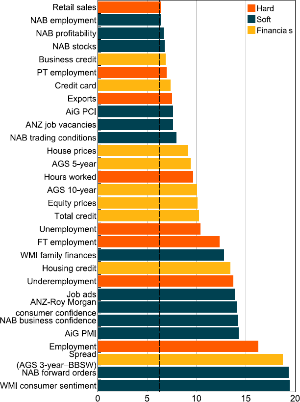
Note: Dashed line represents the critical value = 6.25.
Sources: ABS; Ai Group; ANZ; Authors' calculations; Bloomberg; CoreLogic; NAB; RBA; Westpac and Melbourne Institute.
Notes: GDP is first release. Dashed lines represent 95 per cent confidence intervals.
A.2 Additional MAI estimation details
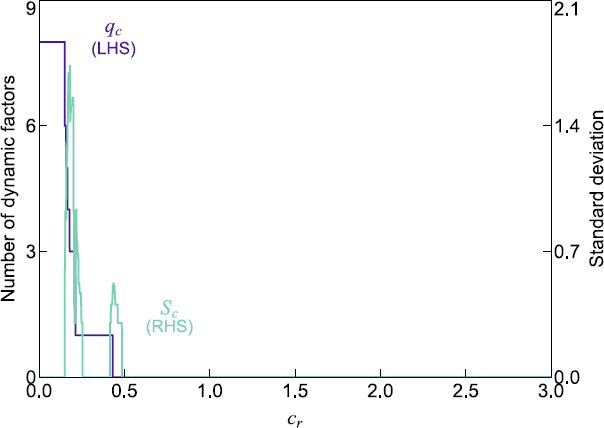
The number of dynamic factors is determined by looking for the second ‘region of stability’ in relation to Sc (i.e. a value of 0) and checking which value of qc this corresponds to. See Hallin and Liška (2007) for more details.
Sources: Ai Group; Authors' calculations; NAB; RBA; Westpac and Melbourne Institute.
Note: Grey lines represent the underlying ‘targeted predictor’ dataset; blue line represents the MAI.
Appendix B: Additional Modelling Results
References
Anthonisz M (2021), ‘Daily Nowcasting of Global and Australian GDP Growth’, Economic research article, Queensland Treasury Corporation website, 26 May, viewed 10 January 2023. Available at <https://www.qtc.com.au/institutional-investors/news-and-publications/research/daily-nowcasting-of-global-and-australian-gdp-growth/>.
Armesto MT, KM Engemann and MT Owyang (2010), ‘Forecasting with Mixed Frequencies’, Federal Reserve Bank of St. Louis Review, 92(6), pp 521–536.
Aruoba SB, FX Diebold and C Scotti (2009), ‘Real-time Measurement of Business Conditions’, Journal of Business & Economic Statistics, 27(4), pp 417–427.
Australian Treasury (2018), ‘Nowcasting Australia's Gross Domestic Product’, Treasury Working Paper No 2018-04.
Aylmer C and T Gill (2003), ‘Business Surveys and Economic Activity’, RBA Research Discussion Paper No 2003-01.
Bai J, E Ghysels and JH Wright (2013), ‘State Space Models and MIDAS Regressions’, Econometric Reviews, 32(7), pp 779–813.
Bai J and K Li (2016), ‘Maximum Likelihood Estimation and Inference for Approximate Factor Models of High Dimension’, The Review of Economics and Statistics, 98(2), pp 298–309.
Bai J and S Ng (2008), ‘Forecasting Economic Time Series Using Targeted Predictors’, Journal of Econometrics, 146(2), pp 304–317.
Bai J and P Wang (2015), ‘Identification and Bayesian Estimation of Dynamic Factor Models’, Journal of Business & Economic Statistics, 33(2), pp 221–240.
Bair E, T Hastie, D Paul and R Tibshirani (2006), ‘Prediction by Supervised Principal Components’, Journal of the American Statistical Association, 101(473), pp 119–137.
Bańbura M, D Giannone, M Modugno and L Reichlin (2013), ‘Now-casting and the Real-time Data Flow’, in G Elliott and A Timmermann (eds), Handbook of Economic Forecasting: Volume 2A, Handbooks in Economics, North Holland, Amsterdam, pp 195–237.
Bańbura M and M Modugno (2014), ‘Maximum Likelihood Estimation of Factor Models on Datasets with Arbitrary Pattern of Missing Data’, Journal of Applied Econometrics, 29(1), pp 133–160.
Bańbura M and G Rünstler (2007), ‘A Look into the Factor Model Black Box: Publication Lags and the Role of Hard and Soft Data in Forecasting GDP’, European Central Bank Working Paper Series No 751.
Barigozzi M and M Luciani (2019), ‘Quasi Maximum Likelihood Estimation and Inference of Large Approximate Dynamic Factor Models via the EM Algorithm’, Unpublished manuscript, ver 1, 10 October. Available at <https://arxiv.org/abs/1910.03821v1>.
Baumeister C and P Guérin (2020), ‘A Comparison of Monthly Global Indicators for Forecasting Growth’, NBER Working Paper No 28014.
Boivin J and S Ng (2006), ‘Are More Data Always Better for Factor Analysis?’, Journal of Econometrics, 132(1), pp 169–194.
Bok B, D Caratelli, D Giannone, A Sbordone and A Tambalotti (2017), ‘Macroeconomic Nowcasting and Forecasting with Big Data’, Federal Reserve Bank of New York Staff Report No 830.
Brillinger DR (1981), Time Series: Data Analysis and Theory, Expanded edn, Holden-Day Series in Time Analysis, Holden-Day, San Francisco.
Bulligan G, M Marcellino and F Venditti (2015), ‘Forecasting Economic Activity with Targeted Predictors’, International Journal of Forecasting, 31(1), pp 188–206.
Chauvet M and S Potter (2013), ‘Forecasting Output’, in G Elliott and A Timmermann (eds), Handbook of Economic Forecasting: Volume 2A, Handbooks in Economics, North Holland, Amsterdam, pp 141–194.
Chinn MD, B Meunier and S Stumpner (2023), ‘Nowcasting World Trade with Machine Learning: A Three-step Approach’, NBER Working Paper No 31419.
Choi H and H Varian (2012), ‘Predicting the Present with Google Trends’, Economic Record, 88(s1), pp 2–9.
Clark TE and MW McCracken (2005), ‘Evaluating Direct Multistep Forecasts’, Econometric Reviews, 24(4), pp 369–404.
Clements MP and AB Galvão (2008), ‘Macroeconomic Forecasting with Mixed-frequency Data: Forecasting Output Growth in the United States’, Journal of Business & Economic Statistics, 26(4), pp 546–554.
Clements MP and AB Galvão (2009), ‘Forecasting US Output Growth Using Leading Indicators: An Appraisal Using MIDAS Models’, Journal of Applied Econometrics, 24(7), pp 1187–1206.
Cunningham A, J Eklund, C Jeffery, G Kapetanios and V Labhard (2012), ‘A State Space Approach to Extracting the Signal from Uncertain Data’, Journal of Business & Economic Statistics, 30(2), pp 173–180.
Doz C, D Giannone and L Reichlin (2011), ‘A Two-step Estimator for Large Approximate Dynamic Factor Models Based on Kalman Filtering’, Journal of Econometrics, 164(1), pp 188–205.
Doz C, D Giannone and L Reichlin (2012), ‘A Quasi–Maximum Likelihood Approach for Large, Approximate Dynamic Factor Models’, The Review of Economics and Statistics, 94(4), pp 1014–1024.
Ferrara L and C Marsilli (2019), ‘Nowcasting Global Economic Growth: A Factor-augmented Mixed-frequency Approach’, The World Economy, 42(3), pp 846–875.
Forni M, M Hallin, M Lippi and L Reichlin (2000), ‘The Generalized Dynamic-factor Model: Identification and Estimation’, The Review of Economics and Statistics, 82(4), pp 540–554.
Foroni C and M Marcellino (2014), ‘A Comparison of Mixed Frequency Approaches for Nowcasting Euro Area Macroeconomic Aggregates’, International Journal of Forecasting, 30(3), pp 554–568.
Foroni C, M Marcellino and C Schumacher (2015), ‘Unrestricted Mixed Data Sampling (MIDAS): MIDAS Regressions with Unrestricted Lag Polynomials’, Journal of the Royal Statistical Society Series A: Statistics in Society, 178(1), pp 57-82.
Galvão AB (2013), ‘Changes in Predictive Ability with Mixed Frequency Data’, International Journal of Forecasting, 29(3), pp 395–410.
Galvão AB and M Lopresto (2020), ‘Real-time Probabilistic Nowcasts of UK Quarterly GDP Growth Using a Mixed-frequency Bottom-up Approach’, Economic Statistics Centre of Excellence, ESCoE Discussion Paper No 2020-06.
Ghysels E, V Kvedaras and V Zemlys (2016), ‘Mixed Frequency Data Sampling Regression Models: The R Package midasr’, Journal of Statistical Software, 72(4), pp 1-35.
Ghysels E, P Santa-Clara and R Valkanov (2004), ‘The MIDAS Touch: Mixed Data Sampling Regression Models’, Centre Interuniversitaire de Recherche en Analyse des Organisations, Scientific Series, CIRANO Working Paper No 2004s-20.
Ghysels E, A Sinko and R Valkanov (2007), ‘MIDAS Regressions: Further Results and New Directions’, Econometric Reviews, 26(1), pp 53-90.
Giannone D, L Reichlin and D Small (2008), ‘Nowcasting: The Real-time Informational Content of Macroeconomic Data’, Journal of Monetary Economics, 55(4), pp 665-676.
Gillitzer C and J Kearns (2007), ‘Forecasting with Factors: The Accuracy of Timeliness’, RBA Research Discussion Paper No 2007-03.
Gillitzer C, J Kearns and A Richards (2005), ‘The Australian Business Cycle: A Coincident Indicator Approach’, RBA Research Discussion Paper No 2005-07.
Hallin M and R Liška (2007), ‘Determining the Number of Factors in the General Dynamic Factor Model’, Journal of the American Statistical Association, 102(478), pp 603-617.
Hartigan L and M Wright (2023), ‘Monitoring Financial Conditions and Downside Risk to Economic Activity in Australia’, Economic Record, 99(325), pp 253-287.
He C and T Rosewall (2020), ‘The Sahm Rule: A Recession Indicator for Australia’, Unpublished manuscript, Reserve Bank of Australia, 16 January.
Higgins P (2014), ‘GDPNow: A Model for GDP “Nowcasting”’, Federal Reserve Bank of Atlanta Working Paper 2014-7.
Jardet C and B Meunier (2022), ‘Nowcasting World GDP Growth with High-frequency Data’, Journal of Forecasting, 41(6), pp 1181-1200.
Kamber G, J Morley and B Wong (2018), ‘Intuitive and Reliable Estimates of the Output Gap from a Beveridge-Nelson Filter’, The Review of Economics and Statistics, 100(3), pp 550-566.
Koenig EF, S Dolmas and J Piger (2003), ‘The Use and Abuse of Real-time Data in Economic Forecasting’, The Review of Economics and Statistics, 85(3), pp 618-628.
Leboeuf M and L Morel (2014), ‘Forecasting Short-term Real GDP Growth in the Euro Area and Japan Using Unrestricted MIDAS Regressions’, Bank of Canada Discussion Paper No 2014-3.
Lee K, N Olekalns, K Shields and Z Wang (2012), ‘Australian Real-time Database: An Overview and an Illustration of its Use in Business Cycle Analysis’, Economic Record, 88(283), pp 495–516.
Lewis DJ, K Mertens, JH Stock and M Trivedi (2021), ‘High-frequency Data and a Weekly Economic Index during the Pandemic’, in WR Johnson and G Herbert (eds), AEA Papers and Proceedings, Vol 111, American Economic Association, Nashville, pp 326–330.
Luciani M (2020), ‘Common and Idiosyncratic Inflation’, Board of Governors of the Federal Reserve System Finance and Economics Discussion Series No 2020-024.
Marcellino M and C Schumacher (2010), ‘Factor MIDAS for Nowcasting and Forecasting with Ragged-edge Data: A Model Comparison for German GDP’, Oxford Bulletin of Economics and Statistics, 72(4), pp 518–550.
Maroz D, JH Stock and MW Watson (2021), ‘Comovement of Economic Activity during the Covid Recession’, Bendeim Center for Finance Princeton University, Working Paper, 15 December. Available at <https://www.princeton.edu/~mwatson/wp.html>.
Matheson TD (2006), ‘Factor Model Forecasts for New Zealand’, International Journal of Central Banking, 2(2), pp 169–237.
McCracken MW (2007), ‘Asymptotics for Out of Sample Tests of Granger Causality’, Journal of Econometrics, 140(2), pp 719–752.
Mosley L, T-ST Chan and A Gibberd (2024), ‘The Sparse Dynamic Factor Model: A Regularised Quasi-maximum Likelihood Approach’, Statistics and Computing, 34, Article 68.
Nunes LC (2005), ‘Nowcasting Quarterly GDP Growth in a Monthly Coincident Indicator Model’, Journal of Forecasting, 24(8), pp 575–592.
Panagiotelis A, G Athanasopoulos, RJ Hyndman, B Jiang and F Vahid (2019), ‘Macroeconomic Forecasting for Australia Using a Large Number of Predictors’, International Journal of Forecasting, 35(2), pp 616–633.
Richardson A, T van Florenstein Mulder and T Vehbi (2021), ‘Nowcasting GDP Using Machine-learning Algorithms: A Real-time Assessment’, International Journal of Forecasting, 37(2), pp 941–948.
Roberts I and J Simon (2001), ‘What do Sentiment Surveys Measure?’, RBA Research Discussion Paper No 2001-09.
Sahm C (2019), ‘Direct Stimulus Payments to Individuals’, in H Bousheym, R Nunn and J Shambaugh (eds), Recession Ready: Fiscal Policies to Stabilize the American Economy, The Brookings Institution, Hamilton Project, Washington DC, pp 67–92.
Schorfheide F and D Song (2015), ‘Real-time Forecasting with a Mixed-frequency VAR’, Journal of Business & Economic Statistics, 33(3), pp 366–380.
Sheen J, S Trück and BZ Wang (2015), ‘Daily Business and External Condition Indices for the Australian Economy’, Economic Record, 91(S1), pp 38–53.
Siliverstovs B (2020), ‘Assessing Nowcast Accuracy of US GDP Growth in Real Time: The Role of Booms and Busts’, Empirical Economics, 58(1), pp 7–27.
Stock JH and MW Watson (2002), ‘Forecasting Using Principal Components from a Large Number of Predictors’, Journal of the American Statistical Association, 97(460), pp 1167–1179.
Stock JH and MW Watson (2016), ‘Dynamic Factor Models, Factor-augmented Vector Autoregressions, and Structural Vector Autoregressions in Macroeconomics’, in JB Taylor and H Uhilg (eds), Handbook of Macroeconomics: Volume 2A, Handbooks in Economics, Elsevier, Amsterdam, pp 415–525.
Stone A and S Wardrop (2002), ‘Real-time National Accounts Data’, RBA Research Discussion Paper No 2002-05.
West KD (2006), ‘Forecast Evaluation’, in G Elliott, CWJ Granger and A Timmermann (eds), Handbook of Economic Forecasting: Volume 1, Handbooks in Economics 24, Elsevier, Amsterdam, pp 99–134.
Copyright and Disclaimer Notice
RP Data Pty Ltd Trading as CoreLogic Asia Pacific Disclaimer Notice
This publication contains data, analytics, statistics, results and other information licensed to the Reserve Bank of Australia by RP Data Pty Ltd trading as CoreLogic Asia Pacific (CoreLogic Data).
© Copyright 2024. RP Data Pty Ltd trading as CoreLogic Asia Pacific (CoreLogic) and its licensors are the sole and exclusive owners of all rights, title and interest (including intellectual property rights) subsisting in the CoreLogic Data reproduced in this publication. All rights reserved.
The CoreLogic Data provided in this publication is of a general nature and should not be construed as specific advice or relied upon in lieu of appropriate professional advice.
While CoreLogic uses commercially reasonable efforts to ensure the CoreLogic Data is current, CoreLogic does not warrant the accuracy, currency or completeness of the CoreLogic Data and to the full extent permitted by law excludes all loss or damage howsoever arising (including through negligence) in connection with the CoreLogic Data.
Acknowledgements
We are grateful to Sarah Hunter, Adrian Pagan, Matthew Read, Kalvinder Shields and John Simon, as well as seminar participants at: CAMA/CAMP Workshop at the University of Sydney (November 2023), the Reserve Bank of Australia (July 2023); the Melbourne Institute (June 2023); the University Rovira i Virgili (January 2022); the Sydney Macroeconomic Reading Group Workshop (June 2021); the 2021 Australian Conference for Economists (July 2021); and the ABS Methodology Division Seminar Series (December 2020) for helpful comments and suggestions. We would also like to thank Paula Drew for editorial and publication assistance and Anthony Richards for encouragement and inspiration. We acknowledge important contributions from Angus Moore and Joyce Tan during the early development of this work and Calvin He for implementing the Sahm rule for Australia. Hartigan also acknowledges partial funding support provided by the Australian Research Council (DP230100959). Any remaining errors are solely our own. The views expressed in this paper are those of the authors and do not necessarily reflect the views of the Reserve Bank of Australia.
Footnotes
The University of Sydney [*]
Economic Analysis Department, Reserve Bank of Australia [**]
The actual publication date was 2 September 2020 (see <https://www.abs.gov.au/statistics/economy/national-accounts/australian-national-accounts-national-income-expenditure-and-product/jun-2020>). [1]
The JobKeeper scheme was a wage subsidy for businesses introduced in March 2020 by the Australian Government to support the economy during the COVID-19 crisis. [2]
For a comprehensive review of DFMs, see Stock and Watson (2016) and references therein. Examples where DFMs have been used in policy institutions include: Matheson (2006); Aruoba, Diebold and Scotti (2009); Cunningham et al (2012); Bańbura and Modugno (2014); Higgins (2014); Bok et al (2017); and more recently, Lewis et al (2021). [3]
The method proposed by Stock and Watson (2002) uses principal components analysis (PCA) while the method developed by Forni et al (2000) uses dynamic PCA. [4]
That is, using higher frequency information to predict the current value of an (unpublished) lower frequency variable. [5]
They focused on quarterly data covering the period 1960 to 2005 and produced forecasts using a recursive scheme for growth in GDP, non-farm GDP, private final demand, household final consumption expenditure with horizons from 2, 4 and 8 quarters ahead. The benchmark model was an AR(1) process. [6]
Australian Treasury (2018) follows the Federal Reserve Bank of Atlanta's ‘GDPNow’ methodology (Higgins 2014) which uses a parametric model based on a state-space model to estimate the DFM. In contrast, Panagiotelis et al (2019) estimate a static factor model by PCA. To predict GDP, they use the factor-augmented (i.e. diffusion index) model approach of Stock and Watson (2002). [7]
Australian Treasury (2008) estimates a monthly factor initially but converts this to a quarterly frequency for use in bridging equations. Panagiotelis et al (2019) converts all monthly series in their dataset to quarterly before extracting any factors. Both implement temporal aggregation by taking the average of the three months in each quarter. [8]
Anthonisz (2021) is an exception and considers mixed frequency data in his analysis. [9]
For a non-exhaustive list, see Clements and Galvão (2008, 2009), Galvão (2013), Foroni and Marcellino (2014), Leboeuf and Morel (2014), Schorfheide and Song (2015), Ferrara and Marsilli (2019), Galvão and Lopresto (2020), Siliverstovs (2020), Baumeister and Guérin (2020), and Jardet and Meunier (2022). [10]
Bai and Wang (2015) define a true DFM as one that incorporates dynamics between the observed series and the factors. See Section 2 for more details. [11]
For MIDAS, see Ghysels, Santa-Clara and Valkanov (2004) and Ghysels, Sinko and Valkanov (2007). For unrestricted MIDAS see Foroni, Marcellino and Schumacher (2015) and for factor augmented MIDAS see Marcellino and Schumacher (2010), Ferrara and Marsilli (2019) and Jardet and Meunier (2022). [12]
Curiously, except for Anthonisz (2021), none of the previous studies in Australia conducted examinations comparing predictive accuracy using formal statistical tests. [13]
The reason this is a problem relates to the size of the common component. If too many noisy series are included in the dataset, then the average common component will be smaller than permitted by asymptotic theory. [14]
Bair et al (2006) proposed an idea akin to hard thresholding, calling their procedure ‘supervised principal components’. They follow similar steps to Bai and Ng (2008), but instead of using the t-statistic to decide which series to retain, Bair el al (2006) retain series with coefficient estimates exceeding a threshold in absolute value (with the threshold value determined by cross validation). [15]
See Doz, Giannone and Reichlin (2011, 2012), Bańbura et al (2013) and Bańbura and Modugno (2014). These authors show that the inclusion of disaggregated data does not deteriorate the performance of the DFM. [16]
For example, an important and timely metric of activity is the Labour Force Survey (LFS) which began in February 1978. [17]
Until June quarter 2020, Australia had not experienced a recession (using the technical definition of two consecutive quarters of negative quarterly GDP growth) since the early 1990s. [18]
The alternative method Bai and Ng propose, soft thresholding, is not suitable for our dataset since the algorithms employed to rank series (i.e. LARS, LASSO or the elastic net) require a balanced dataset. [19]
A criticism of hard thresholding suggested by Bulligan et al (2015) is that it tends to select highly collinear predictors. This is because hard thresholding only takes account of the bivariate relationship between the target variable and each predictor in isolation and does not account for the information contained in other predictors. However, it is not really a problem and more likely to be a benefit. Boivin and Ng (2006), Bair et al (2006), Bai and Ng (2008) and Jardet and Meunier (2022) all show that forecast accuracy improves by selecting fewer but more informative predictors. One possible reason for this finding suggested by Boivin and Ng (2006) is that reducing the number of variables can help concentrate the factor structure and enable more efficient estimation. [20]
In all our analyses we work with the compound growth rate of first-release real GDP. [21]
This is the same as the mixed frequency distributed lag model of Koenig et al (2003) and the unrestricted MIDAS model of Foroni et al (2015). [22]
The number of indicator variables were determined by examining individual t-statistics. All but the indicator for 2021:Q1 were significant at the 5 per cent level. [23]
Unlike Bai and Ng (2008), we do not include lags of the dependent variable as additional controls since ACF/PACF plots for quarterly GDP growth suggest there is no statistically significant autocorrelation (see Figure A3). [24]
In comparison, monthly datasets in the United States and Europe typically have hundreds of series to consider. [25]
Using the stricter 5 per cent significance level resulted in 24 series being selected, which we felt was too small as it was at the lower end of the range of 20 to 40 variables suggested by Panagiotelis et al (2019). [26]
The minimum sample size suggested by Bai and Ng (2008) relates to the PCA-based method for estimating factor models. This is not the method we use to estimate the DFM (in Section 2.2). However, our method is identical to both Bańbura et al (2013) and Australian Treasury (2018) and Monte Carlo exercises of Doz et al (2011, 2012) show substantial robustness to misspecification is achieved by this method even with a small number of variables. [27]
A third source of dynamics that is sometimes considered involves allowing the idiosyncratic processes to be autocorrelated. We do not allow for this as the dynamics in the factors will be sufficient to account for the dynamics in the data. [28]
Bai and Wang (2015) regard the specification to be a static factor model when there are no lags in the measurement equation (i.e. s = 0). Luciani (2020) is another example that also implements a DFM with dynamic factor loadings. [29]
Estimation is ‘quasi’-maximum likelihood because the model is misspecified. This comes from assuming that R, the covariance matrix of the idiosyncratic component, is diagonal. Further, we also assume that both noise processes are Gaussian. However, in large samples, this misspecification has been shown to be no issue to consistently estimating the factors and factor loadings (see Doz et al (2012), Bai and Li (2016) and Barigozzi and Luciani (2019)). [30]
The number of dynamic factors is determined by looking for the second ‘region of stability’ in relation to Sc and checking which value of qc this corresponds to. [31]
This is because the likelihood function of our model is invariant to any invertible linear transformation of the factors. That is, for any invertible matrix H the parameters and are observationally equivalent and hence is not identifiable from the data. To achieve identifiability of , we need to impose an identifying restriction. [32]
Three versions of the MAI are available once all the parameters have been estimated using the QMLE procedure. These include the predicted, filtered, and smooth estimates. In our analysis we will only focus on the filtered estimate of the MAI following Sheen et al (2015), who state that the filtered estimate (based on the full sample parameter estimates) is appropriate for conditional forecasting, while the smoothed estimate is appropriate for within-sample estimation. [33]
For the United States, the Sahm rule signals a recession when the three-month moving average of the national unemployment rate rises by a ½ percentage point or more relative to its low during the previous twelve months. [34]
Series from the soft data category are also most correlated with the MAI, as shown by the magnitude of the dynamic loadings for the top ten ranked series in Figure A5. [36]
To test statistical significance, we regress the squared difference series on a constant and compute the t-statistic for the constant term using a long-run variance estimator. The t-statistic is 0.11 while the p-value is 0.91. [37]
In addition, Richardson, van Florenstein Mulder and Vehbi (2021) for New Zealand; however, Anthonisz (2021) is an exception. [38]
MIDAS regression implements a form of temporal aggregation, but unlike using the average for example, the weights used by the model are entirely determined by the data. For an introduction to MIDAS regression for macroeconomic prediction see Armesto, Engemann and Owyang (2010). [39]
In this approach, quarterly GDP growth is included as an extra observable in the measurement equation in Equation (2) when estimating the factor model specified with monthly frequency data. This interpolates quarterly GDP growth across the three months in quarter. [40]
In most cases, the state-space model was a little more accurate, but it is also computationally more demanding. [41]
In related work, Schorfheide and Song (2015) show that predictions of real US GDP growth from a mixed frequency VAR model are empirically similar to those obtained from an (unrestricted) MIDAS regression. [42]
This allows for greater flexibility in how the weights used in temporal aggregation are determined by the data and is reminiscent of the mixed frequency distributed lag method introduced earlier by Koenig et al (2003). [43]
However, when the difference in frequencies is large, Foroni et al (2015) find that R-MIDAS outperforms U-MIDAS. [44]
In their analysis the authors also compared a two-step approach (first estimate monthly factors and then estimate the forecast of quarterly GDP growth using a FA-MIDAS model) to an integrated approach (estimate monthly factors and then forecast using a state-space model). They conclude that the two approaches produce similar forecasts, and therefore supports the findings of Bai et al (2013) and our decision to focus on MIDAS models instead of a state-space framework. Further, the best performing model in many cases was found to be a simple MIDAS structure without a distributed lag term and only one lag of the latent factors. [45]
As noted by Clements and Galvão (2009), there are two ways of using vintage data to estimate a model in real time. First, use the ‘end-of-sample’ vintage. In this case, for each t the most current vintage data are used to estimate the model. Second, use ‘real-time’ vintage data. Under this approach, for each t the initially available data are used to estimate the model. This approach was introduced by Koenig et al (2003) to overcome an issue with the first method. The problem is that any given vintage of data will be a combination of first releases, partially revised and fully revised data. Koenig et al claim that model parameters estimated using the first method will be inconsistent. Importantly, the results of Koenig et al and Clements and Galvão (2008) suggest the real-time vintage method produces more accurate predictions of output growth in the United States using distributed lag and MIDAS models. [46]
A notable exception is Panagiotelis et al (2019), who only consider current vintage data in their work. [47]
This is also comparable to Koenig et al (2003) in relation to forecasting US quarterly GDP growth and Galvão and Lopresto (2020) in relation to nowcasting UK quarterly GDP growth. [48]
The steps we follow to estimate the real-time MAI is as follows. First, we estimate all the parameters of the model using the QMLE method. Second, we take the final parameter estimates and re-run the Kalman filter again using those parameter values and the targeted predictor dataset. [49]
All estimation was done in R using the ‘midasr’ package of Ghysels, Kvedaras and Zemlys (2016). [50]
As already noted, the BIC ranks the U-MIDAS model with six lags second in terms of model suitability. [51]
Predictions made using M3 are sometimes labelled as ‘backcasts’, that is, those that are backwards looking or that are made (shortly) after the end of the quarter of interest (see Siliverstovs (2020) and Chinn, Meunier and Stumpner (2023), who both use the same four-period horizon). [52]
This MIDAS model framework is reminiscent of Koenig et al (2003) and Leboeuf and Morel (2014), who both also use fixed model specifications in their work. [53]
The QA model is a special type of R-MIDAS model in which the weights are constrained to be uniform (i.e. equal to 1/3 in each month). Further, uniform weights are equivalent to the normalised exponential Almon function with the first parameter set to 1 and the rest set to 0 and the normalised beta function with all parameters set to 1. [54]
One exception is Chinn et al (2023), who also do not find a uniform improvement in accuracy as more information becomes available when nowcasting world trade volumes using a similar four-horizon setting. [55]
Note that an RMSE close to one implies the uncertainty in the model's prediction is comparable to the variability of quarterly GDP growth since the unconditional sample standard deviation of quarterly growth is approximately one over the sample period we work with. [56]
Simulations conducted in Clark and McCracken (2005) show that MSE-F bootstrap critical values yield better size results compared to those based on asymptotic critical values. West (2006) also recommends using the bootstrap when testing for differences in MSEs between nested models. Additionally, Clark and McCracken (2005) show the MSE-F test is more powerful than t-type counterparts (such as the DMW test). The reason for this is because, under the alternative hypothesis, the F-type test statistic diverges to infinity at a faster rate. [57]
In this way the trajectories are generated under the null hypothesis the nesting models have similar accuracy as the benchmark sample mean model. [58]
Note, the null is never rejected for the sample mean and AR(1) models, indicating that there really is no statistical difference between the two models. [59]
Anthonisz (2021) is the only study using Australian data that is comparable to our work; however, his focus was nowcasting year-ended (annual) GDP growth. [60]