RDP 2015-10: The Life of Australian Banknotes 4. ‘Feige’ Steady-state Method
August 2015 – ISSN 1448-5109 (Online)
- Download the Paper 1.22MB
Some currency issuers use variants of the steady-state formula to overcome some of the biases inherent in the traditional steady-state method. One limitation of the traditional steady-state method is that it is adversely affected by the growth in the number of circulating banknotes. This stems from the fact that destructions (the denominator) tend to reflect banknotes that were issued some time ago, whereas the stock of banknotes on issue (the numerator) reflects the cumulative sum of many years of issued banknotes, including those that have only recently been issued. In other words, the average age of banknotes on issue falls if the population is growing due to the addition of new banknotes. Clearly this distortion in the banknote life estimates has the greatest effect on denominations that survive the longest in circulation and those that experience the fastest growth rates in demand.
Feige (1989) derives an alternative formula for average banknote life by comparing the number of times a banknote can typically be used in transactions in its lifetime to the number of times it is handled per year.

With some algebra, and assuming that the total number of transactions in a typical banknote's lifetime does not change over time, he provides a simple formula for banknote life.[7] With reference to Figure 1, this formula is calculated as c divided by the average of d and a.
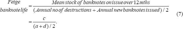
Since this method assumes that the hazard rate is constant over time, the median life of banknotes can still easily be calculated. By including data on new banknote issuance, the formula can reduce the bias in Equation (5) by taking into account the growth in banknotes on issue.[8] As expected, the resulting mean and median banknote life estimates are somewhat lower than the traditional steady-state results (Tables 4 and 5; Figure 4).
| Denomination | Paper 1985–91 | NNS polymer 2000–14 | |||
|---|---|---|---|---|---|
| Steady state | Feige | Steady state | Feige | ||
| $5 | 0.7 | 0.7 | 6.3 | 5.3 | |
| $10 | 0.8 | 0.7 | 6.0 | 5.4 | |
| $20 | 1.1 | 1.1 | 6.9 | 6.5 | |
| $50 | 2.2 | 2.0 | 17.4 | 15.5 | |
|
Sources: Author's calculations; RBA |
|||||
| Denomination | Paper 1985–91 | NNS polymer 2000–14 | |||
|---|---|---|---|---|---|
| Steady state | Feige | Steady state | Feige | ||
| $5 | 0.5 | 0.5 | 4.4 | 3.7 | |
| $10 | 0.5 | 0.5 | 4.1 | 3.7 | |
| $20 | 0.7 | 0.7 | 4.8 | 4.5 | |
| $50 | 1.5 | 1.4 | 12.0 | 10.7 | |
|
Sources: Author's calculations; RBA |
|||||
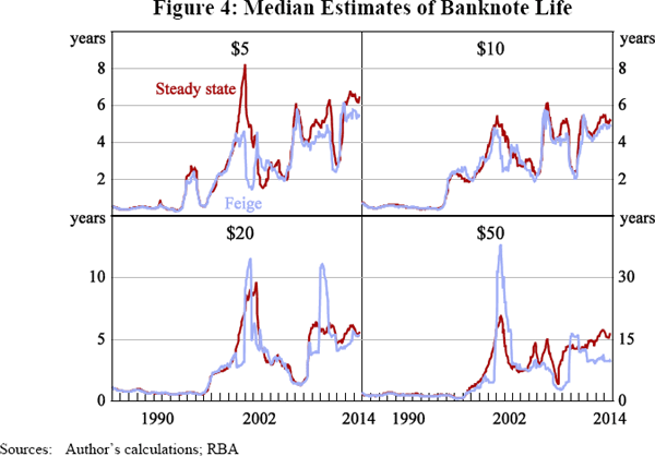
Although the results of the Feige equation were found to be less volatile for the paper series and the low-value $5 and $10 polymer banknotes, there were still some sharp fluctuations in the higher-denomination polymer banknote data (Table 6; Figure 4). One of the key causes is that the Feige equation only accounts for new banknotes when they are initially introduced into circulation. As such, the Feige method is less suitable for situations where banknotes are temporarily withdrawn from circulation. For example, in the period leading up to Y2K, large volumes of new banknotes were issued to meet precautionary demand and were withdrawn once they were no longer required, to be reissued at a later time. As a result, there was a sharp decline in the estimated banknote life in 1999 and a sharp increase a year later.
| Denomination | Paper 1985–91 | NNS polymer 2000–14 | |||
|---|---|---|---|---|---|
| Steady state | Feige | Steady state | Feige | ||
| $5 | 0.12 | 0.08 | 2.3 | 1.8 | |
| $10 | 0.11 | 0.08 | 1.5 | 1.4 | |
| $20 | 0.21 | 0.18 | 3.0 | 3.6 | |
| $50 | 0.32 | 0.26 | 4.9 | 10.0 | |
|
Sources: Author's calculations; RBA |
|||||
Footnotes
See Appendix A for the derivation of the formula. [7]
Continuing the previous analogies to animals, in effect this formula attempts to control for changing demographics in a population by including both ‘births’ and ‘deaths’. [8]