RBA Annual Conference – 1992 Discussion
1. Kunio Okina
The paper by Blundell-Wignall, Lowe and Tarditi gives an excellent summary of inflation indicators, as well as interesting empirical evidence about their nature in the Australian economy.
I will focus my remarks on the role of asset prices, money, and credit as indicators, partly because the scope of the paper is too broad to allow comments on all the interesting points, and also because comparing the Japanese experience since the mid-1980s in terms of asset prices and money with the Australian experience is fruitful for this Conference.
(a) Asset Prices as Indicators
As in Australia, asset prices in Japan are statistically poor leading indicators of inflation.
As shown in Figure 1, stock prices continued to rise until the end of 1989, and then declined sharply. Land prices have shown a similar trend. These movements are consistent with the movement of M2 plus CDs, the monetary aggregate which the Bank of Japan has emphasised most, though they are not reflected in either the rate of inflation (as measured by the CPI) or the GNP deflator.
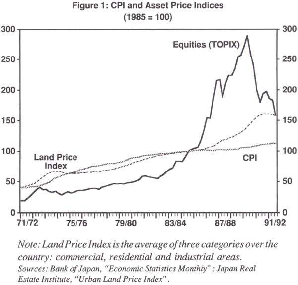
In Japan, many believe that the sharp rise in asset prices in the late 1980s and subsequent crash was merely the result of overly optimistic expectations with respect to the economy, or what has been termed a speculative bubble, at that time. Many market participants were too optimistic. Nevertheless, I think this interpretation may be too simplistic. As shown in Figure 2, during the period from when the yen appreciated strongly, after the Plaza Agreement in 1985, to when world stock prices sharply declined, after “Black Monday” in 1987, interest rates in Japan remained quite low. Thus, the trend of Japanese asset prices from the mid-1980s can largely be explained by the movement of interest rates.
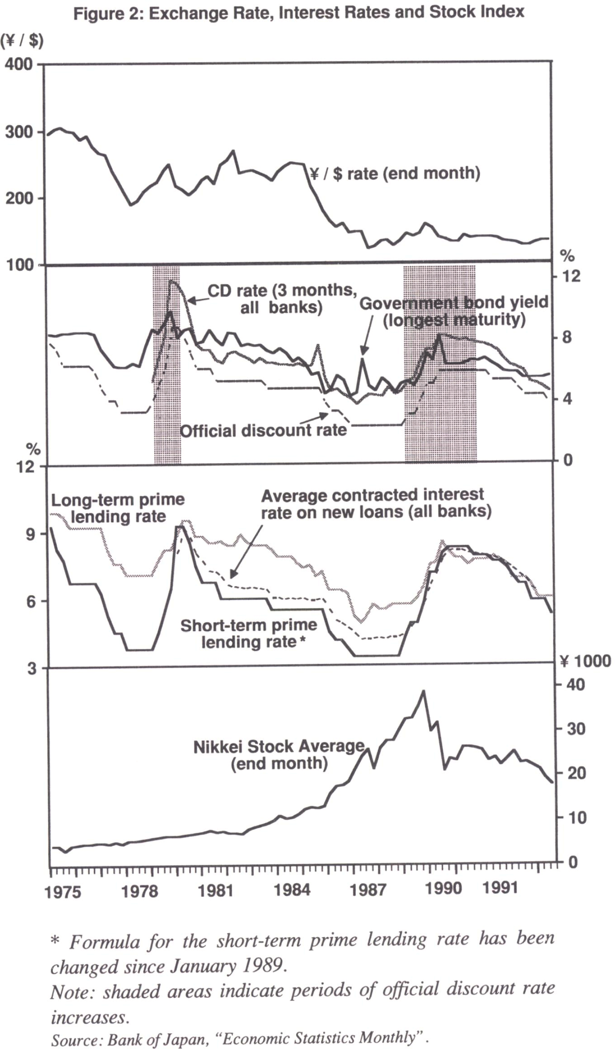
However, in spite of the fact that interest rates began to rise from mid-1989, stock prices continued to increase until the end of the year. Though corporate current profits were high during this period, stock prices evidently overshot their fundamental values for more than half a year.
The paper by Blundell-Wignall and his colleagues argues that “asset price movements driven by market inefficiency should be transitory … deviate from fundamentals for a time before reverting back again”. The point here is how long such transitory periods last. If they persist, say, for more than half a year, then it might not be prudent to rely overly upon asset prices as inflation indicators.
A related question is why asset prices tend to overshoot fundamentals. Perhaps excessive optimism, or “tulip mania” type expectations with respect to market participants, are only part of the answer, and there may be some structural factors creating market inefficiencies which amplify the degree of overshooting in asset markets.
In Australia, incomes policy might have played an important role in this respect. In the case of Japan, however, there is no incomes policy. Instead, there are several structural factors. For example, banks and other business corporations do not sell their stocks even when stock prices rise sharply. The cross-holding of stock among companies is one structural reason for this behavior. But, at the same time, the tax system may act as a disincentive to sell. Namely, unrealised capital gains are untaxed. Thus, banks and firms prefer to keep them as hidden reserves. Land prices are also affected by inheritance tax and other regulations.
To utilise asset prices as indicators, the influence of the cross-holding of stock, the tax system, and other structural factors influencing asset prices in each country should be examined carefully.
(b) Money and Credit as Indicators
Next, I will discuss money and credit. Blundell-Wignall and his colleagues argue that, in Australia, broadly-defined money has demonstrated a reasonable leading relationship with major swings in inflation except in late 1988 and 1989. Credit growth also leads major turning points in inflation, including the most recent deflationary period.
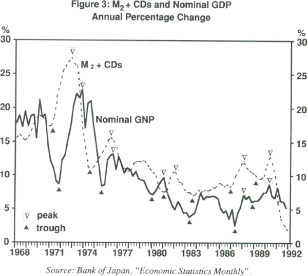
The situation is somewhat different in Japan. As seen in Figure 3, recent turning points with respect to M2 plus CDs do not lead turning points of nominal GNP (or the CPI). In addition, as shown in Table 1, simple maximum cross-correlation coefficients between inflation-related indicators and M2 plus CDs became smaller in the 1980s with incredibly long leads. The performance of narrowly-defined money deteriorates as well.
Part of the reason for these results is the shift of funds within and from bank deposits to assets outside the money supply, especially “teigaku chokin” postal saving deposits (Figure 4), a ten-year time deposit, which can be withdrawn without penalty after six months.
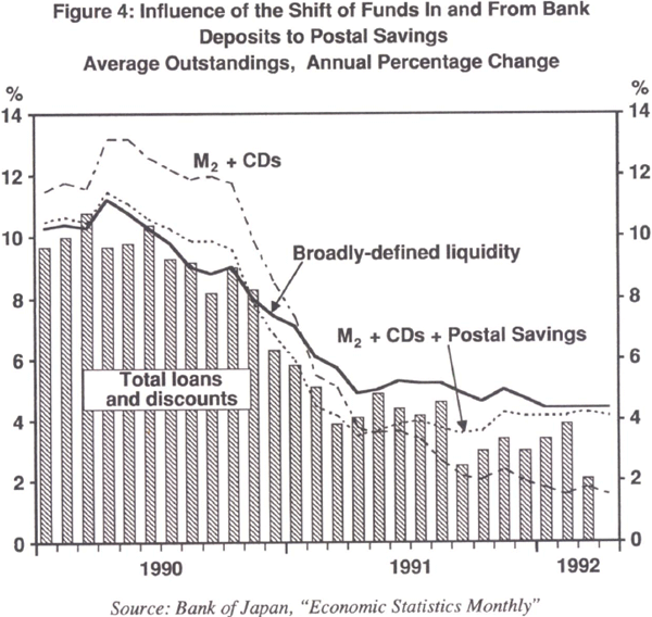
If we look at broadly-defined money in which postal savings deposits are included, the lead time is still reasonable even in the 1980s, but the maximum cross-correlation coefficients are fairly small (Table 1).
As was suggested by Blundell-Wignall and his colleagues for the case of Australia, credit aggregates also seem to perform a little bit better in Japan if we use broader aggregates. Maximum cross-correlation coefficients are higher and the lead time is reasonable.
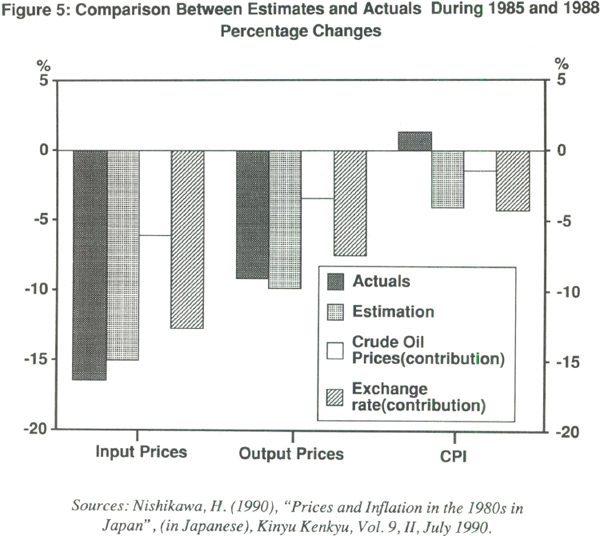
One reason why the relationship between M2 plus CDs and inflation became weak can be found in the large real shocks of the mid-1980s. From 1985 to 1988, M2 plus CDs kept growing fairly rapidly, but the yen's appreciation after the Plaza Agreement in 1985 and the oil price decline, due to the so-called oil glut, put strong downward pressure on inflation. Figure 5 provides an example of the estimation of this effect on prices, as surveyed by staff of the Bank of Japan, using Leontief's classical input-output table. This estimation suggests that if there had been inflationary pressure from the monetary side at that time, it could easily have been offset by the real shocks of the yen's appreciation and the fall in oil prices.
One interesting point here, as I indicated earlier, is that although the relationship between M2 plus CDs and inflation weakened in the 1980s, the relationship between M2 plus CDs and asset prices in Japan was not lost.
| M1 | M1′ | M1′+CDs | M2 | M2+CDs | M3+CDs | Broadly-Defined Liquidity | C0 | C1 | C2 | C3 | |
|---|---|---|---|---|---|---|---|---|---|---|---|
| WPI | (−4)0.90 | (−4)0.83 | (−4)0.83 | (−5)0.89 | (−5)0.89 | (−5)0.88 | (−5)0.86 | (−4)0.83 | (−4)0.81 | (−4)0.93 | (−4)0.88 |
| CPI | (−5)0.91 | (−6)0.81 | (−6)0.81 | (−6)0.89 | (−6)0.89 | (−5)0.91 | (−6)0.85 | (−6)0.93 | (−5)0.92 | (−5)0.92 | (−5)0.91 |
| GNP Deflator | (−5)0.91 | (−5)0.86 | (−5)0.86 | (−6)0.94 | (−6)0.94 | (−5)0.94 | (−5)0.90 | (−5)0.94 | (−5)0.93 | (−5)0.92 | (−5)0.95 |
| Nominal GNP | (−4)0.85 | (−4)0.90 | (−4)0.90 | (−5)0.93 | (−5)0.93 | (−4)0.91 | (−4)0.91 | (−4)0.94 | (−3)0.93 | (−3)0.91 | (−4)0.89 |
| Equity Prices | (+2)0.83 | (−2)0.86 | (+2)0.86 | (+1)0.84 | (+1)0.84 | (+1)0.67 | (+1)0.85 | (+2)0.78 | (+2)0.74 | (+2)0.68 | (+2)0.72 |
| Land Prices | (−2)0.79 | (−2)0.87 | (−2)0.87 | (−2)0.86 | (−2)0.86 | (−2)0.81 | (−2)0.89 | (−2)0.83 | (−2)0.75 | (0)0.68 | (−2)0.75 |
| WPI | (−11)0.67 | (−11)0.66 | (−11)0.58 | (−11)0.74 | (−10)0.67 | (−4)0.57 | (−3)0.35 | (−13)0.37 | (−3)0.54 | (−8)0.64 | (−3)0.60 |
| CPI | (−12)0.61 | (−11)0.61 | (−11)0.56 | (−12)0.81 | (−12)0.72 | (−8)0.65 | (−5).0.51 | (−14)0.31 | (−8)0.67 | (−8)0.63 | (−4)0.77 |
| GNP Deflator | (−12)0.39 | (−11)0.39 | (−10)0.37 | (−10)0.42 | (−9)0.50 | (−10)0.58 | (−3)0.37 | (−11)−0.03 | (−8)0.67 | (−9)0.51 | (−4)0.63 |
| Nominal GNP | (−10)0.68 | (−10)0.67 | (−9)0.65 | (−2)0.19 | (−3)0.30 | (−3)0.28 | (−2)0.24 | (−11)0.54 | (−1)0.48 | (−4)0.45 | (−3)0.41 |
| Equity Prices | (−2)0.41 | (+3)0.80 | (+2)0.82 | (+4)0.78 | (+3)0.80 | (+3)0.64 | (+2)0.61 | (+3)0.83 | (+4)0.59 | (+3)0.63 | (+2)0.25 |
| Land Prices | (−6)0.60 | (−2)0.80 | (−2)0.76 | (0)0.85 | (0)0.76 | (0)0.59 | (0)0.35 | (−2)0.64 | (0)0.65 | (0)0.84 | (0)0.15 |
| Notes: All variables are year-to-year changes; M1 =
Cash currency in circulation + deposit money; M1′ = M1 + Quasi-money of private corporations; M1′ + CDs =MV + Certificates of deposit of private corporations; M2 = M1 + Quasi money; M2 + CDs = M2 + Certificates of deposit; M3 + CDs = M2 + CDs + Deposits (including CDs) of Post Offices and Agricultural Cooperatives, Fishery Cooperatives, Credit Cooperatives, Labor Credit Associations + Money Trusts and Loan Trusts of all Banks; Broadly defined liquidity = M3 + CDs + Bonds with repurchase agreement + Bank debentures + Government bonds + Investment trusts + Money deposited other than money in trust + Foreign bonds; C0 = Lendings of All Banks on a domestic basis (including trust accounts); C1 = C0 + Lendings of Shinkin Banks, The Norin chukin Bank, The Shoko Chukin Bank, Credit Federations of Agricultural Cooperatives, Credit Federations of Fishery Cooperatives, Foreign Banks, Government Financial Institutions†, and Other Financial Institutions†; C2 = Outstanding of domestic fund procurement by corporate business and personal sectors; C3 = C2 + Outstanding of domestic fund procurement by public sector; (−X) indicates maximum cross correlation is attained when ‘Money’ leads ‘inflation’ by X quarters. * Government Financial Institutions include Japan Development Bank, Export Import Bank of Japan, The Housing Loan Corporation, Hokkaido and Tohoku Development Corporation, The Japan Finance Corporation for Municipal Enterprises, The Small Business Finance Corporation, The People's Finance Corporation, and The Agriculture, Forestry and Fisheries Finance Corporation. † Other Financial Institutions include Life Insurances, Non Life Insurances, Credit Cooperatives, and Labor Credit Associations. Sources: Bank of Japan, ‘Economic Statistics Monthly’; Japan Real Estate Institute, ‘Urban Land Price Index’. |
|||||||||||
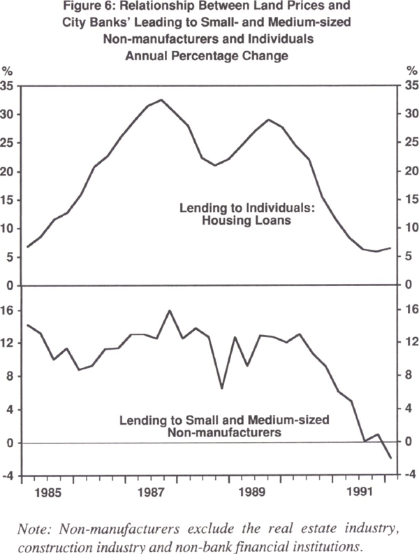
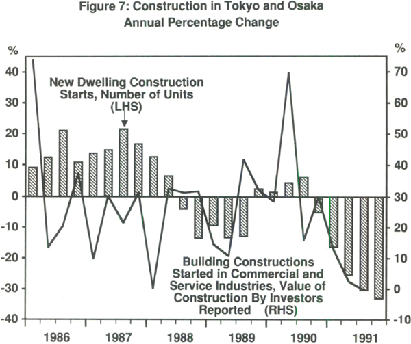
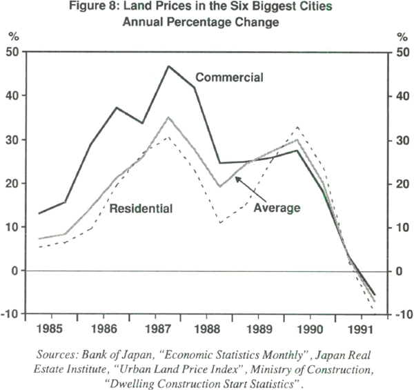
Again, as shown in Table 1, stock prices and land prices are either leading or simultaneous indicators of M2 plus CDs. There are many possible reasons for this. On the one hand, the demand for money is possibly influenced by wealth effects stemming from high asset prices; on the other hand, the amount of bank lending, especially housing loans and loans to small- and medium-sized non-manufacturers, has responded to the movement of land prices, as is shown in Figures 6, 7 and 8.
(c) Implications
These are our experiences of asset prices, credit, and money as inflation indicators in Japan during the 1980s. I think there are at least three implications consistent with the paper by Blundell-Wignall and his colleagues.
First, financial market liberalisation and innovation are likely to affect the demand for narrower aggregates much more than for very broad aggregates. Thus, in Japan, even M2 plus CDs might be too narrow thus far in the 1990s.
Second, broader credit aggregates may be a better indicator of inflation than monetary aggregates, but further investigation of this proposition is still needed.
Third, since monetary aggregates are significantly affected by asset prices, when asset prices and inflation diverge, the movement of monetary aggregates may not be a good indicator of inflation with respect to goods and services.
2. Mervyn King
This paper is a reduced form empirical investigation into the transmission mechanism of monetary policy. Given the lack of a coherent theoretical framework for understanding the transmission mechanism, an investigation of this kind can add a great deal to our understanding of the impact of monetary policy on inflation. I found this an interesting paper which struck a chord with me in its analysis of the use of indicators for setting monetary policy. For many years we have had cause to resort to ‘long and variable time lags’ in our description of the transmission, and these lags appear to have become longer and more variable. There is a demonstrable need for leading indicators not just for the real economy, but also for the inflation rate.
At the outset, one might pose the question of whether the focus of an empirical investigation should be on the construction of an intermediate target or on targeting inflation directly. For example, if one were successful in identifying a number of indicators of future inflation then they might be combined together, in a way that I shall describe below, to construct a synthetic intermediate target. Changes in monetary policy could, then, be related to the latest observed value of the intermediate target. Alternatively, a vector autoregression could be used to form a prediction of inflation, and the setting of the policy instrument be made a function of the difference between predicted inflation and the current target. The results of this paper could be used in either way.
It is helpful to start by considering the univariate time series behaviour of the inflation rate. The authors estimate such a model for the inflation rate, and from these estimates one can infer a measure of the degree of persistence of inflation. Table 1 pulls together estimates of the persistence of inflation from three of the papers presented at this Conference. It can be seen that Australia and the United States share a high degree of persistence, whereas Germany and Japan exhibit a much lower degree of persistence. What do these estimates tell us? In the absence of a theoretical framework for the transmission mechanism they are not easy to interpret. They are clearly reduced-form rather than structural estimates. And I was not wholly persuaded by the authors that one should interpret these results as the outcome of adaptive expectations on the part of economic agents. Graph 1 shows that even the within sample one-step-ahead forecasts miss most of the turning points in inflation. I would rather interpret these results in terms of expectations on the future policy stance of the authorities. In Germany and Japan there is greater credibility that the authorities will take whatever measures are necessary to bring inflation down quickly. There is less credibility that inflation will be brought down as rapidly in either the United States or Australia. But these estimates do show that in all countries there is danger in accommodating inflation. Unless inflation is quickly nipped in the bud it may persist and become even more difficult to bring down, and incur a higher subsequent cost. There is wisdom in Charles Goodhart's recommendation that the authorities stand ready to adjust monetary policy quickly and to learn from past experience of the danger of acting too little and too late.
| (Sum of AR coefficients) | |
|---|---|
| Taylor72:4 – 91:3 | |
| (Table 1, sums of log coefficients) | |
| US | 0.88 |
| Germany | 0.64 |
| Japan | 0.64 |
| Blundell-Wignall et.al. 67:4 – 91:4 | |
| (Table 2, Column 2) | |
| Australia | 0.87 |
| Stevens 62:1 – 91:4 | |
| (Table 5, Row 1) | |
| Australia | 0.76 |
Before turning to the empirical estimates, I would like to make three points about the estimation of the vector autoregressions. First, one would doubt that they exhibit parameter stability because they are likely to depend upon the policy regime pursued by the authorities. This is clearly the lesson of Goodhart, Lucas, and Bill Phillips. Nevertheless, these regressions can be helpful because they suggested that one might use Bayesian updating of the regressions to form optimal forecasts of future inflation. Second, the paper presents tests only on the hypothesis that the sum of the coefficients on the lagged indicator variables is zero. Although this statistic is interesting, it would also be appropriate to present the standard Granger-causality test, which is an F-test of the joint hypothesis that each individual coefficient for each lag is zero. Even if the sum of the coefficients on all of the lags equals zero, a particular lag of a variable could be a good predictor of inflation.[1] Third, it would be interesting to see the results when more than one regressor were included in the same autoregression. This may run into the problem of the number of degrees of freedom, but when the indicators contain different information and are not independent of each other bias may result from the purely univariate approach.
The paper presents the results for four different types of indicator variable:
- real variables;
- money and credit aggregates;
- asset prices; and
- the yield curve.
I would make only three brief comments here. First, predictions of inflation can be sensitive to estimates of the output gap. In the paper the output gap is estimated using a Hodrick-Prescott filter. Results are presented for two values of the parameter that penalises lack of smoothness in the estimated filter. But it would be helpful to see the results presented for a simple linear time trend (the case when λ tends to infinity). I am only too well aware that in the United Kingdom estimates of the degree of downward pressure on inflation are highly sensitive to whether or not potential output is following a linear time trend or whether it is affected by a recession. Second, results for the United Kingdom suggest also that a broad credit aggregate has greater information content than a broad monetary aggregate. Of course, in general both aggregates have information content, and perhaps should be combined. Third, the finding that the yield curve is a predictor of future inflation suggests that it would be useful to present results of a univariate regression of inflation on lagged values of short-term interest rates. This would give the reduced-form lag structure between the policy instrument itself and the ultimate objective. Again one doubts that parameter stability would obtain, but as a benchmark the results would be helpful.
In one sense this paper suggests that monetary policy must be set in an eclectic fashion. More than one indicator contains useful information about the impact of monetary policy on inflation, and the challenge is to know which indicators are relevant in any period and to combine the information contained in them. It is hard to disagree with this view. But I think there is more that could be done to model formally the process by which the information content of different aggregate indicators is combined together. In principle, the weight attached to any given indicator should reflect the relative variances in the link from the indicator to the inflation rate. In general, covariances would also need to be taken into account, but this would provide a way of trying to weight together different indicator variables.
In the debate between discretion and rules, the paper comes down firmly on the side of discretion. But is this enough? Is there not a choice between total discretion, on the one hand, and a little less discretion, on the other. I am sympathetic to the view expressed in John Taylor's paper that it is helpful, at the very least influencing the expectations of economic agents, to provide a little more substance to the framework within which monetary policy decisions are made. I do not suggest that this is easy. And it may be that the appropriate direction to pursue is the one suggested by Charles Goodhart – namely that the authorities should be given more discretion over the choice of setting of monetary instruments, and the indicators which they use to reach those decisions, but should experience less discretion over the objectives of monetary policy. An intermediate target is, therefore, replaced by an inflation objective. It is up to the central bank to decide how best to meet that objective, but if the inflation objective is not met then pre-set penalties would be imposed on the central bank. As a potential recipient of this discipline, I can imagine many difficulties with it. But it is then up to central banks to provide a more coherent view of how discretion in the setting of monetary policy will be exercised.
3. General Discussion
The discussion of the Blundell-Wignall et al. paper focused on four main areas:
- rules versus discretion in responding to indicators of inflation pressure;
- the implications of the persistence of inflation for the conduct of monetary policy;
- the role of the Accord in affecting asset price indicators; and
- the relative usefulness of credit as an indicator.
With regard to rules versus discretion, a number of speakers made the point that the central lesson of the paper was that it is important to pay attention to leading indicators if monetary policy is to act pre-emptively to control inflation. It was also recognised that indicators always needed to be interpreted within the context of unique factors influencing the current business cycle, and that their relative usefulness might vary over time. This meant that there certainly needed to be considerable discretion in the way indicators are interpreted when forecasting inflation. It was also pointed out that discretion in the use of indicators is entirely consistent with giving monetary policy the task of targeting low inflation. Some suggested that a rule specifying how policy reacts to deviations from the low inflation target was important. Others argued that specific rules would be inappropriate. Reactions to ex post inflation would be too late, and hence more costly in terms of activity. Since leading indicators are unlikely to have a stable relationship with inflation, it would also be unwise to include them in any rigid reaction function.
The consistent finding that there was considerable persistence in Australian inflation dynamics also attracted a number of comments. With regard to explaining the phenomenon, it is not necessary to appeal to backward-looking price expectations. Persistence could also be explained by rational expectations in circumstances where prices are slow to adjust to changes in monetary policy. Some participants argued that a high degree of inflation persistence suggested the need for a quick response by authorities to the onset of inflationary pressure. The failure to raise interest rates sufficiently sharply would be costly in terms of the degree to which inflation persists over time.
With respect to the Accord, it was acknowledged that it did hold wage pressures in the late 1980s, and hence probably helped reduce the cost of disinflation. But it was also pointed out that the Accord could not have held wage pressure indefinitely if monetary policy had not been tightened. In terms of its implications for interpreting indicators, it was widely accepted that holding inflation through incomes policy in the face of strong demand would cause pressures to emerge elsewhere in the economy. Since profits were affected, this probably did contribute to asset price inflation over and above that attributable to monetary policy and asset market trends in other countries. Such additional factors underline why it is not appropriate for monetary policy to target asset prices. They may be a useful guide for policy, however, provided the other factors are taken into account.
There was some discussion about the link between credit, nominal income and inflation. It was argued that, historically, nominal income has led credit in Australia. However, in a system with deregulated financial markets, credit may have some leading indicator properties (though not causal) for nominal income. In these circumstances, it should not be surprising that credit might be an unambiguous leading indicator of inflation itself, which adjusts more slowly than real activity.
Footnote
This statistic was calculated and available to the authors prior to the conference, but was not included in Tables 2 and 3. The statistics are included in the published version for completeness – editor. [1]