RBA Annual Conference – 1992 Inflation, Indicators and Monetary Policy Adrian Blundell-Wignall, Philip Lowe and Alison Tarditi[*]
1. Introduction
The aim of this paper is to provide a context for discussion of the role of indicators of inflation pressure in the conduct and transmission of monetary policy in Australia. It does not specifically discuss the issue of what the ultimate objective for monetary policy should be. Rather, it is taken as given that the principal objective is to achieve and maintain low inflation over some reasonable period of time. The paper argues that monetary policy decisions need to be made in a pre-emptive fashion to avoid unnecessary swings in economic activity. This need arises out of the fact that while inflation exhibits a strong pro-cyclical component, it often lags the cycle. In this environment, monetary policy decisions depend crucially on how leading indicators are assessed.
Some indicators of inflation pressure are largely exogenous to monetary policy. In this respect it is important to bear in mind that Australia is a small, commodity-exporting, country. As a price-taker in world commodity markets, the terms of trade are subject to large exogenous shifts, which impact on real income, prices and the exchange rate. Other useful indicators are more directly related to the transmission mechanisms of monetary policy itself. If changes in monetary policy succeed in altering the outlook for future inflation, variables directly linked with the way monetary policy works should be affected ahead of inflation outcomes. Here it is important to note that, in line with a number of other countries, Australian financial markets were completely liberalised during the 1980s. This has important on-going implications for monetary policy, which now must rely on influencing the economy through market mechanisms rather than constraints arising from official regulations.
The paper reviews empirical evidence about the nature of indicators of inflation. It pays specific attention to those indicators which reflect the monetary transmission mechanism in an economy characterised by liberalised financial markets and periodic exogenous shifts in the terms of trade. Section 2 outlines why indicators are important for monetary policy decisions and how they relate to the assumed transmission mechanisms. Section 3 reviews a subset of indicators that are of particular interest to monetary policy decision making. Section 4 examines some puzzling features of the role of indicators in the tightening and easing of monetary policy in the late 1980s and early 1990s. Section 5 concludes.
2. Indicators and Monetary Policy
(a) Why Indicators?
If goods prices were determined in the same way as financial auction prices, and adjusted instantaneously to changes in policy-determined interest rates, the setting of monetary policy would be straightforward. Policy could be used to achieve any desired price level immediately, without any effect on output, and prices could be monitored continuously on electronic screens. Goods prices are, however, not set in such markets. Prices are ‘sticky’ for a variety of reasons, information is incomplete and markets are not perfect. The result of these imperfections is that changes in monetary policy impact on both activity and prices, as do various exogenous real shocks. These effects do not occur instantaneously, but are drawn out over long periods of time. As a result, monetary policy has an important role in interacting with other factors in the evolution of the business cycle. A role for indicators derives from the need to do this in a timely way.
(i) The Pro-cyclical Component of Inflation and Inertia
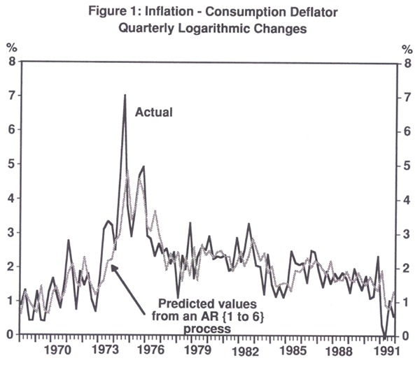
Inflation rates are often characterised by significant persistence, which makes current rates highly correlated with past rates. This persistence is often referred to as ‘inertia’. Explanations for inertia in the theoretical literature include staggered wage and price setting in conjunction with credibility problems concerning the willingness of authorities to reverse inflation surprises (Taylor (1979) and Ball (1990)). Thus, if a supply shock causes prices to rise and economic agents expect inflation to be accommodated, these expectations would be built into current wage negotiations and price setting. Alternatively, price expectations may be partly adaptive. In Australia's case this seems plausible. Figure 1 shows inflation measured by the consumption deflator and a prediction based on an autoregressive equation estimated with six quarterly lags. If expectations were based on past inflation, they would have predicted current rates of change of prices rather well.
The inertia in inflation means that nominal demand pressures determined by monetary policy are typically reflected first in economic activity. While it has been a central lesson of the past couple of decades that there is no positive long-run trade-off between activity and inflation, it is still the case that there is an important short-run pro-cyclical component to inflation. As activity rises above potential, excess demand pressures gradually cause inflation to accelerate. If activity declines relative to potential, there will be downward pressure on inflation. The business cycle therefore modifies the momentum in inflation, but it often does so with a lag. This is illustrated in Table 1, which compares peaks and troughs in activity, measured by the gap between actual and potential real GDP, with peaks and troughs in inflation, measured by the four-quarter-ended percentage change in the consumption deflator. The activity variable typically leads inflation by between two and seven quarters.
| Peak in Output Gap | Peak in Inflation | Lag (quarters) |
|---|---|---|
| June 1970 | September 1971 | 5 |
| September 1973 | March 1975 | 7 |
| March 1979 | June 1980 | 5 |
| June 1981 | September 1982 | 5 |
| September 1985 | March (or December) 1986 |
2 (or 5) |
| March 1990 | No peak | – |
| Trough in Output | Trough in Inflation | Lag (quarters) |
| December 1967 | September 1969 | 7 |
| March 1972 | December 1972 | 3 |
| December 1977 | September 1978 | 3 |
| June 1983 | December 1985 | 6 |
| June 1986 | No trough | – |
| Note: The output gap is calculated with a Hodrick-Prescottfilter as in section III. See also Figure 2. Inflation is calculated as the four-quarter-ended percentage change in the consumption deflator. | ||
The inertia and pro-cyclical components to inflation imply important trade-offs in the conduct of monetary policy. Monetary tightening to bring inflation down is likely to result in a weakening of real demand and output for a time. Conversely, easy monetary policy can promote stronger growth in the short term, but with the risk of allowing inflation to accelerate later. These trade-offs are less favourable, the greater is the inertia in inflation. Since inertia appears to be important in Australia, it is essential that monetary policy should not accommodate major deviations from the low-inflation objective. Once inflation is permitted to rise, and becomes built into backward-looking expectations, costs in terms of economic activity to reduce it cannot be avoided.
(ii) Problems with Intermediate Targets
One view of how monetary policy should be conducted to minimise these problems involves the setting of an intermediate target for either the money supply or exchange rate. This view is predicated on the argument that the long and variable lags associated with monetary policy make it of limited use as a countercyclical tool. As a result, it downgrades the use of indicators, preferring instead to achieve the ultimate goal of low inflation through a simple rule.
Some of the problems with this view are addressed in more detail by Goodhart (1992). He emphasises the well-known proposition that monetary targets need not generate price stability if the money demand function is subject to unexpected shifts. The unpredictable impact of financial deregulation on Australian monetary aggregates in the 1980s is well documented elsewhere.[1] While it is to be hoped that shocks of this magnitude will not be repeated in the 1990s, the prospect of monetary aggregates playing the role they played prior to liberalisation does not seem great if the evidence from other countries is anything to go by. In general, as the number of assets with characteristics similar to money have multiplied, and as banks have paid market rates to attract funds, motives for holding money have become similar to those for holding other components of wealth. At the same time, the transactions motive has weakened. International evidence suggests that these developments have often seen the disappearance of any causal relationship from money to nominal demand and inflation in the short run. In many instances, even longer-run relationships have broken down.[2] It was for these sorts of reasons that monetary targeting was significantly downgraded in most countries that liberalised their financial markets during the 1980s.
Analogous problems arise for exchange rate targets. Such targets only deliver low inflation if (i) the anchor country can be relied upon to achieve this goal; and (ii) the domestic economy is not subject to important real shocks different from those experienced in the anchor country. Goodhart (1992) points out some of the problems in both respects with the anchor role of Germany in the European Monetary System (EMS) at present. With regard to Australia, the important point to note is that, as a commodity exporter, the terms of trade vary considerably more than in other major OECD countries, and often inversely. Fixing or even managing the exchange rate in the face of such real shocks is a highly inefficient approach to achieving a low-inflation outcome. Allowing the exchange rate to change in response to these real shocks is an important part of the adjustment process. Fixing the exchange rate forces more of the adjustment onto activity and inflation in the short-run.[3]
(iii) The Pre-emptive Adjustment of Monetary Policy
An alternative approach involves adjusting the levers of monetary policy pre-emptively to achieve and maintain a low-inflation outcome directly, thus bypassing the need for an intermediate target. Leading indicators are indispensable for conducting policy in this way, since judgments have to be made about the future course of inflation rather than its current rate. Given the strong inertia in inflation, current monetary policy actions influence actual outcomes with a long lag. Failure to act pre-emptively risks new trends in the price level becoming built into expectations, thus exacerbating the cyclical costs associated with inflation control. Some practical examples are instructive.
From a starting point of low inflation, signs of excessive growth in nominal demand require pre-emptive tightening to reduce the extent to which actual increases in prices become built into expectations. Prompt action early on should forestall the need for stronger action later. Even real shocks such as terms of trade or productivity changes may require some response from monetary policy. In principle, price adjustment in these cases is actually desirable as a part of the normal ‘equilibrating’ process. Such adjustments should, therefore, be seen as a level shift in prices and not as increases in inflation. However, if price level increases are confused with inflation, and expectations are partly adaptive, a change in the price level may well be translated into expectations of higher inflation. In this case there is an argument to tighten monetary policy to offset the inflation implications of real shocks.
Conversely, in a situation in which tight monetary policy is being used to reduce inflation, decisions must be made as to when it is appropriate to begin the process of easing prior to the point where ‘low’ inflation is achieved. Nominal interest rates must certainly be permitted to fall in line with the decline in expected inflation. These reductions, however, still leave real interest rates at the high levels which initiated the process of disinflation. Thus, in addition, real interest rates also need to decline as inflation begins to approach ‘desired’ levels. If these declines do not occur, the downturn in economic activity would be prolonged to an unnecessary degree. An easing of policy that permits an economic recovery does not mean that progress in lowering inflation will stop, or be reversed. Indeed, the economy can be permitted to grow faster than potential output growth before full capacity is reached. While always diminishing during the recovery phase, the gap will nevertheless continue to bear down on inflation for some time after the easing has commenced, while relative prices (real interest rates, real exchange rates and real unit labour costs) adjust back towards levels more consistent with the requirements of sustainable longer-run growth.
Thus, having the principal objective of monetary policy as the achievement and maintenance of low inflation is not a sufficient guide for short-run decisions about how the levers of policy should be set in practice. The fundamental analytical problem for monetary policy decision making is that, in addition to the long and variable lags, it is, a priori, difficult to distinguish between trend and cycle in the inflation rate and between shifts in price levels and inflation. The practical problem is to decide how much policy should be adjusted now to ensure inflation, over some reasonable horizon, is consistent with objectives. Therefore, the practical implementation of monetary policy should depend heavily on:
- the use of indicators of where inflation is likely to move in the absence of any changes in the levers of policy, i.e. to permit pre-emptive changes should they be required; and
- some understanding of the effects of any changes to policy on the level of short-run real activity, in the first instance, and inflation some time later on.
(b) Which Indicators?
Implicit in the above discussion is a view of the way economies operate that has been dubbed the ‘mainstream central bank model’ (Friedman (1990)). The most important characteristic of this ‘model’ is that while there may be no positive long-run trade-off between the level of activity and inflation, short-run prices are responsive to conditions in labour and goods markets. Moreover, prices adjust slowly, and price expectations are at least partly adaptive. It follows that past inflation trends and the position of the economy in relation to potential output are likely to be important indicators of future inflation pressure. Specific measures of these variables are therefore given considerable attention in the empirical analysis in section 3 of the paper.
The other main indicators studied in section 3 were chosen because of their role in the transmission mechanism of monetary policy, as it is assumed to operate in liberalised financial markets. Monetary policy impacts on nominal interest rates in the first instance, and real interest rates are also affected because of sticky prices and the partly backward-looking nature of inflation expectations. These interest rate changes affect activity and (later) inflation:
- by influencing the exchange rate, since the interest differential with other countries is affected;
- by causing spending plans to be delayed or brought forward (intertemporal substitution) which is observed in (though not ‘caused’ by) the prior behaviour of credit aggregates; and
- by inducing wealth effects through changes in asset prices (equity, residential property, and commercial property prices) which are determined by expectations about discounted future returns.
In addition to these indicators, the behaviour of some monetary aggregates is also examined, even though their role is likely to be less useful following financial deregulation.
Two particular characteristics of the Australian economy complicate these standard transmission mechanisms. First, incomes policy (the Accord) was used extensively during the 1980s and early 1990s. This policy tended to weaken the link between activity and wages growth. As a result, the behaviour of wages warrants individual attention as an indicator of inflation. The second factor is Australia's proneness to exogenous swings in the terms of trade. The income and substitution effects induced by rapidly rising export prices tend to create excess demand for non-traded goods. Thus, the terms of trade also warrants specific attention as a leading indicator of inflation.
Finally, the yield curve is of particular interest as a leading indicator, because its slope often reflects the interaction between monetary policy and inflation expectations. Monetary policy actions determine the level of the short-term interest rate (the ‘liquidity’ effect). There is also an inflation expectations component in longer-term interest rates (the ‘Fisher’ effect). Thus a tightening of policy which is expected to reduce activity and future inflation via the above transmission mechanisms will also cause long rates to fall relative to short rates, since future short-term interest rates would be expected to decline.
3. Assessing Alternative Indicators of Inflation
Leading indicators which are useful in assessing future inflation pressures should have at least three important characteristics. First, they should have a statistically significant relationship with the forecast variable. Second, variations in the indicator variable should occur well before variations in the inflation rate.[4] Third, there should be theoretical support for their use as indicators.
It is not necessary for such indicators to have a causal role, although this would be a desirable feature in itself. Indeed, if expectations are forward-looking, expected future inflation may well ‘cause’ the indicator variable – this is of particular relevance to credit, asset prices determined in auction markets, and the yield curve.
Most of the indicators mentioned in section 2 can be used to forecast the rate of inflation itself over various horizons in the future. The slope of the yield curve, however, is somewhat different. It uses the relationship between expected inflation and nominal interest rates to generate differences between expectations of inflation over alternative horizons. Indicators useful for forecasting the inflation rate are considered first. Subsequently, ways in which the yield curve can help in assessing future prospects for inflation are explained and evaluated.
The indicators most likely to be useful for forecasting actual inflation mentioned in section 2 fall into three broad categories:
- real and price indicators: here, the gap between output and potential GDP, the rate of wage inflation, the terms of trade and the rate of change of import prices (which encapsulate exchange rate effects) are considered;
- money supply and credit aggregates: where the growth rates of currency,[5] broad money and total Australian Financial Institutions (AFI) credit are chosen; and
- asset prices: where inflation of equity prices, house prices, commercial property prices and a weighted-average of these three are considered.
The information content of each of these three groups of indicators is tested within a framework that emphasises the temporal ordering of innovations in variables.
One of the key features of the dynamics of inflation mentioned earlier – inertia – is captured by a basic autoregressive forecasting equation for the inflation rate of the form:
where Δp is the rate of inflation, defined to be the quarterly percentage change in the consumption deflator, and ε is a serially uncorrelated error term. Equation [1] is estimated over the period 1967Q2 to 1991Q4. Six lags were necessary to eliminate autocorrelation (AR(6)), and t-values are based on standard errors which are White-corrected for heteroskedasticity. The results are reported in Table 2. Results over a shorter sample period to 1989Q4 are shown in Table 3. Using the full sample period, the sum of the coefficients on past inflation of 0.84 suggests strong positive autocorrelation and is highly significant. Estimated values from this equation were shown in Figure 1. This demonstrates that the past behaviour of inflation provides considerable information concerning the current rate. Similar results are obtained using the shorter sample period.
The strategy adopted to evaluate indicators of inflation from groups (i) to (iii), above, is to see whether they improve the performance of this AR(6) model. That is, each potential indicator is tested to determine what, if any, additional information it possesses about future inflation that is not already accounted for by lagged inflation itself.[6] To this end the following generalised equation is used:
where zt is the additional indicator variable. The null hypothesis is that Σγi = 0, i.e. that the indicator variable does not help in forecasting inflation. Significant t-statistics for the sum of the coefficients indicates rejection of the null hypothesis. Where possible the sample periods are the same as that used for the autoregressive model. These results are also reported for the longer and shorter sample periods in Tables 2 and 3, respectively.
One important problem with forecasting equations that rely on temporal ordering between inflation and changes in indicators is that they may be structurally unstable. The following factors make the period after the 1983 recession one in which there is likely to have been a change in the relationship between inflation and the leading indicators:
- the exchange rate was floated, with the result that it was more likely to be driven by the commodity price/terms of trade cycle;
- financial markets were liberalised, leading to changes in the extent to which liquidity constraints were binding and to shifts in money and credit demand; and
- output grew for a long period in circumstances where wages were contained by the Accord and the profit share rose markedly.
Consequently, the bottom rows of Tables 2 and 3 report chi-squared statistics for tests of the null hypothesis that the sum of the parameters on the indicator variables are the same over the period after 1984Q1 as over the period prior to 1984Q1.
Where indicators are found to provide significant within-sample information for forecasting inflation, their out-of-sample properties are also tested over the period 1990Q1 to 1991Q4. This was a period in which inflation fell from 6.4 per cent, in the twelve months to 1989Q4, to 2.1 per cent, in the twelve months to 1991Q4. Since mechanisms that influence inflation might have quite different weights in different periods, this exercise is of interest because it provides insights into the ex ante interpretation problems faced by monetary authorities at major turning points. Furthermore, to the extent that indicators reflect underlying mechanisms, albeit very imperfectly, it might also provide some insight into the major sources of disinflation over this period.
Out-of-sample forecasts for the indicator models selected in Tables 2 and 3 are reported in Table 4. To facilitate interpretation, the forecasts are presented as four-quarter-ended percentage changes. Three sets of results are presented:
| Variable | Dynamic Forecasts Using Autoregressive Prediction of Exogenous | |||||||||
|---|---|---|---|---|---|---|---|---|---|---|
| 89Q4 | 90Q1 | 90Q2 | 90Q3 | 90Q4 | 91Q1 | 91Q2 | 91Q3 | 91Q4 | RMSE | |
| Actual Outcome | 6.4 | 6.8 | 5.9 | 5.5 | 6.4 | 5.0 | 3.8 | 3.7 | 2.1 | — |
| Autoregressive* | — | 6.0 | 6.5 | 5.9 | 6.0 | 5.9 | 5.8 | 5.6 | 5.6 | .0077 |
| Output gap* | — | 6.4 | 5.9 | 5.7 | 5.4 | 5.4 | 5.0 | 4.8 | 4.9 | .0074 |
| Wages | — | 6.7 | 6.9 | 7.3 | 7.5 | 7.7 | 7.7 | 8.1 | 8.6 | .0127 |
| Terms of trade (TOT)* | — | 6.9 | 6.9 | 7.3 | 7.5 | 7.2 | 7.1 | 6.9 | 7.1 | .0104 |
| TOT and Import prices | — | 6.8 | 6.7 | 7.1 | 7.4 | 7.3 | 7.1 | 7.2 | 7.3 | .0103 |
| Currency | — | 6.1 | 4.9 | 4.0 | 3.3 | 2.9 | 2.8 | 3.0 | 3.6 | .0075 |
| Broad Money* | — | 6.9 | 6.6 | 6.7 | 7.2 | 7.0 | 6.9 | 7.0 | 7.1 | .0096 |
| AFI Credit* | — | 6.8 | 6.0 | 5.9 | 6.1 | 5.8 | 6.0 | 6.1 | 6.1 | .0081 |
| Dynamic Forecasts Using Actual Exogenous Variables | ||||||||||
| 89Q4 | 90Q1 | 90Q2 | 90Q3 | 90Q4 | 91Q1 | 91Q2 | 91Q3 | 91Q4 | RMSE | |
| Actual Outcome | 6.4 | 6.8 | 5.9 | 5.5 | 6.4 | 5.0 | 3.8 | 3.7 | 2.1 | — |
| Autoregressive* | — | 6.5 | 6.0 | 5.9 | 6.0 | 5.9 | 5.8 | 5.6 | 5.6 | .0077 |
| Output gap* | — | 6.8 | 7.1 | 8.0 | 8.7 | 9.3 | 9.2 | 8.7 | 8.4 | .0131 |
| Wages | — | 6.7 | 6.9 | 7.3 | 7.4 | 7.6 | 7.3 | 7.3 | 7.5 | .0113 |
| Terms of trade (TOT)* | — | 6.9 | 6.8 | 7.3 | 7.4 | 7.0 | 6.7 | 6.2 | 6.1 | .0091 |
| TOT and Import prices | — | 6.8 | 6.7 | 6.9 | 7.0 | 6.7 | 6.3 | 5.8 | 5.3 | .0081 |
| Currency | — | 6.1 | 4.9 | 4.1 | 3.4 | 3.4 | 3.8 | 4.8 | 5.7 | .0092 |
| Broad Money* | — | 6.9 | 6.6 | 6.5 | 6.7 | 6.2 | 5.6 | 5.1 | 4.5 | .0065 |
| AFI Credit* | — | 6.8 | 6.0 | 5.9 | 5.8 | 5.3 | 5.1 | 4.6 | 4.1 | .0062 |
| Rolling Horizon Static Forecast (Updating Model) | ||||||||||
| 89Q4 | 90Q1 | 90Q2 | 90Q3 | 90Q4 | 91Q1 | 91Q2 | 91Q3 | 91Q4 | RMSE | |
| Actual Outcome | 6.4 | 6.8 | 5.9 | 5.5 | 6.4 | 5.0 | 3.8 | 3.7 | 2.1 | — |
| Autoregressive* | — | 6.5 | 6.5 | 5.7 | 5.3 | 6.6 | 4.5 | 3.4 | 2.5 | .0078 |
| Output gap* | — | 6.4 | 6.7 | 5.6 | 5.0 | 6.5 | 4.0 | 2.8 | 2.1 | .0084 |
| Wages | — | 6.7 | 7.1 | 5.8 | 5.4 | 6.8 | 4.9 | 3.7 | 3.0 | .0097 |
| Terms of trade (TOT)* | — | 6.9 | 6.8 | 6.0 | 5.2 | 6.4 | 4.5 | 3.3 | 2.4 | .0078 |
| TOT and Import prices | — | 6.8 | 6.7 | 5.9 | 5.3 | 6.5 | 4.5 | 3.6 | 2.2 | .0076 |
| Currency | — | 6.1 | 6.0 | 5.1 | 5.0 | 6.6 | 4.9 | 4.1 | 2.9 | .0092 |
| Broad Money* | — | 6.9 | 6.6 | 5.6 | 5.4 | 6.0 | 4.9 | 3.3 | 1.8 | .0069 |
| AFI Credit* | — | 6.8 | 6.2 | 5.7 | 5.3 | 6.1 | 5.0 | 3.4 | 1.7 | .0071 |
| *Note: Indicates the forecasting equation has its insignificant constant term constrained to zero. | ||||||||||
- The first panel shows dynamic forecasts of the models in Table 3 (estimated to 1989Q4) using a fourth order autoregressive equation to predict the path of the indicator variable over the period 1990Q1 to 1991Q4. This approach gives considerable weight to the observed behaviour of the indicator variable over the course of 1989.
- The second panel shows dynamic forecasts of the models estimated to 1989Q4, but uses the actual path of the indicator variable over the next two years. This essentially assumes that the authorities could predict the indicator variable perfectly, but uses no information about the actual behaviour of inflation.
- The third panel of Table 4 presents out-of-sample rolling-horizon forecasts. The model is estimated to 1989Q4 and is used to forecast 1990Q1. The model is then re-estimated to 1990Q1 and, using information about the outcome for inflation in that quarter, is used to forecast inflation in 1990Q2, and so forth. In this approach the forecast horizon is shorter but, as before, only information available at the time the forecast had to be made is used in the test.
Also shown are the predictions of a naive autoregressive model of the inflation process. This serves as the yardstick against which the various indicator forecasts are compared.
(a) Real and Price Indicators
(i) The Output Gap
Modern business cycle analysis is typically based on the deviation of output from its potential level.[7] The inclusion of such a gap variable in equation [2] can be thought of as a reduced form for the standard expectations-augmented Phillips curve, where expectations are based on past inflation. It is, therefore, not only an indicator in the temporal sense, but also a standard theoretical explanation of inflation – inflation accelerates as the output gap widens. Holding output above trend for a sustained period would see inflation continually accelerating until the gap was closed.
The construction of such a gap variable requires an appropriate trend in activity
to be defined. The method adopted here is that of Hodrick and Prescott (1980);
i.e. computation of the trend component,
 , from the seasonally-adjusted
actual logarithm of real GDP, yt, from the expression:
for an appropriately chosen positive value of λ,. The first term is the sum
of squared deviations of
 from yt,
or the degree of fit of
 . The second term
involves the sum of squares of the trend component's successive differences,
which reflects the degree of smoothness of the trend component. Variations
in the trend growth rate are penalised at the rate λ. The results reported
here are based on λ=1600, the value favoured by Kydland and Prescott
(1990). Monitoring where the economy is in relation to such a trend, and using
high frequency indicators of activity to predict its evolution over time, are
both likely to be important aspects of monetary policy decision making.
Figure 2 shows the output gap and inflation from mid-1967 to the end of 1991. Negative output gaps typically precede troughs in inflation, while positive gaps lead inflationary peaks (see also Table 1). The most notable exception to this relationship was from late 1988 to early 1990, when a positive gap does not appear to have been associated with any pick-up in inflation.[8]
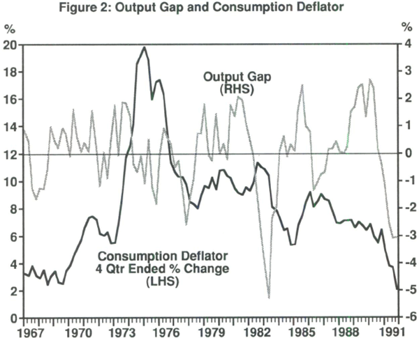
A summary of the estimates of equation [2] including six lags of the output gap over the period 1967 to 1991 is shown in the second column of Table 2. The sum of the coefficients on past lags of inflation at 0.87 remains high, and is well determined, reflecting the strong inertia in the inflation process. The sum of coefficients on lags of the gap variable is 0.15, which is significantly different from zero at the 4 per cent level. When the model is estimated to 1989Q4 (see Table 3), however, the sum of coefficients is much higher, at 0.27, and significant even at the 0.3 per cent level. The null hypothesis of no structural change in the sum of coefficients is rejected for the model estimated to 1991Q4. In contrast, it is not rejected for the model estimated to 1989Q4. This suggests that the output gap's relationship with inflation changed (weakened) only during 1990 and 1991.
The dynamic forecasts using the gap model shown in Table 4 under-predict the slowing of inflation from 1990Q1 to 1991Q4. Here, autoregressive forecasts of the gap perform much better than the actual values because the forecast gap is based on trend output estimated only to 1989Q4. The fact that 1989 was a high point for activity gives rise to a slightly negative gap which is projected forward into 1990 and 1991. Use of the actual large positive output gap in 1989 and 1990 (the panel 2 results) sees inflation accelerate to 9.3 per cent by 1991Q1, before decelerating to 8.4 per cent in 1991Q4. The rolling-horizon forecasts, in contrast, perform well, capturing the full extent of the deflation in 1991 much better than the simple autoregressive model of inflation (equation [1]).
Since the output gap equation can be interpreted as a reduced-form Phillips curve, the dynamic forecasts of relatively high inflation in 1990 and 1991 reflect ex ante wage pressure during 1989/90.[9] That the strength of the economy in 1989 and 1990 did not result in any acceleration of actual inflation, as predicted by the gap model, is consistent with the influence of special factors that temporarily broke the link between demand and wage inflation.
(ii) Wages
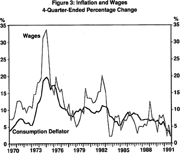
Actual wage and price inflation are shown in Figure 3. Prior to the wage freeze in
1982–83, wages appear to have had a close relationship with consumer
price inflation. Except for the second half of the 1970s, when full or partial
indexation was a factor making for a lagging relationship, wages tended to
lead prices over this period. Since 1983, however, the relationship appears
to have been much looser. Over this period incomes policy via the Accord appears
to have held wages growth at rates fluctuating around an average of about 6
to 7 per cent per annum. During the 1991 recession, wages growth then declined
to less than 5 percent. The temporal ordering tests reported in Table 2 suggest
that average earnings adjusted for hours worked provide some leading information
relevant for forecasting inflation. The sum of coefficients on lagged wages
growth of 0.24 is significantly different from zero at the 1 per cent
level.[10]
However, the coefficient on lagged prices falls significantly compared to other equations,
and the
 is lower than that for the simple autoregressive
model. This suggests that it is unclear whether wages pass the criterion that
they should contain additional information not already accounted for by lagged
inflation itself.
Out-of-sample forecasts for 1990 and 1991 using the wage equation perform very poorly compared with the naive autoregressive model (and all of the other indicators shown in Table 4). The reason for this is that wages growth of 6 to 7 per cent in 1990 affects the inflation forecast for 1991. But the equation does not capture the demand factors contributing to reduced price and wage inflation in 1991. The effect of the Accord in 1989 and 1990, based in large part on wage-tax trade-offs, was to prevent excess demand in goods and labour markets from spilling over into an acceleration of wage and price inflation in the short run, as predicted by the dynamic output gap forecasts.[11] That is, it contained wage outcomes compared to the ex ante wage pressures implied at the time. By so doing, it is arguable that the Accord transferred some of the inflation pressure to other parts of the economy. These results imply, therefore, that wages were probably a less useful guide for monetary policy at the time, compared to those leading indicators to which the inflationary pressures were transferred. This issue is taken up further in Section 4.
(iii) The Terms of Trade and the Exchange Rate/Import Prices<
The terms of trade was emphasised earlier as being an important source of real shocks which affect the Australian economy. While to a very large extent its impact can be thought of as being embodied in the output gap, there are two reasons why it deserves to be investigated as an indicator in its own right. First, major fluctuations in the terms of trade are driven by world commodity prices. The terms of trade are, therefore, a barometer of the level of demand in the rest of the world. In addition, they have a direct impact on domestic demand via the relative price effect. Since both factors affect real demand and prospects for the Australian economy more generally, the terms of trade may be a useful proxy for expected real demand (as opposed to actual outcomes measured by the gap). Second, commodity prices are determined as auction prices and are available on a daily basis. If there is information about expected demand in terms of trade shifts, it would be possible to monitor them at a relatively early stage.
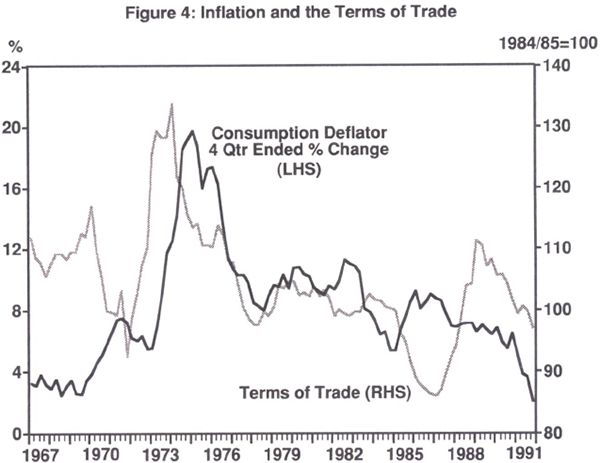
Figure 4 shows inflation and the terms of trade. The terms of trade appears to lead most major turning points in inflation from the late 1960s, with the important exception of the 1985–86 period. At this time, the deterioration of the current account and a rapid rise in foreign debt in response both to the terms of trade decline and the fiscal situation, required a major downward structural adjustment of the nominal and real exchange rate. In fact, the nominal exchange rate fell by a record one third in these years, pushing up import prices (shown in Figure 5) despite a sharp tightening of monetary policy. This unusually large depreciation saw Australian consumer price inflation rise substantially above that of major overseas countries. The recovery of the terms of trade in 1988 and 1989 (as with the output gap) was not associated with increased inflation, as the exchange rate recovered ground at this time and import prices fell, while at the same time ex ante wage pressure was contained by the Accord. In the most recent phase of deflation the terms of trade has again declined, but on this occasion import prices have been relatively stable. Estimates for equation [2] including rates of change of the terms of trade are shown in Table 2. The autoregressive component is still highly significant and the sum of coefficients on lags of the terms of trade, 0.13, is significantly different from zero at the 5 per cent level.
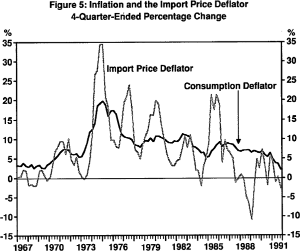
The importance of the exchange rate, through its impact on import prices, as an indicator of inflation pressure is also reported in Table 2. Over the full sample, dominated by fixed or managed exchange rates, the sum of coefficients on lagged import price inflation is not significantly different from zero. One possible reason for this finding is the existence of a strong link between the terms of trade and the exchange rate.[12] Thus changes in the terms of trade have two effects on inflation.
These effects work in opposite directions. As discussed earlier, falls in the terms of trade have a contractionary effect on the economy which acts to reduce inflation. However, with flexible exchange rates, a decline in the terms of trade is likely to be accompanied by a depreciation of the currency, which serves to increase inflation. Thus, controlling for import prices (and hence the exchange rate) should increase the positive leading relationship between the terms of trade and inflation. Similarly, controlling for the terms of trade should see a stronger positive link between past import prices and current inflation.
This proposition is tested by including both the rates of change in the terms of trade and import prices in equation [2]. In this case the sum of lags on the terms of trade is 0.21 and on import prices 0.20 (much larger than their previous individual estimates). Both are significantly different from zero at the 1 per cent level in the Table 2 and 3 results. The structural stability tests suggest a change in the relationship between the terms of trade, import prices and inflation after 1984Q1, presumably because of the change in exchange rate regime. Nevertheless, the results suggest that the terms of trade and the exchange rate should be considered together when assessing the stance of monetary policy. Thus, for example, if the terms of trade was rising sharply and the exchange rate and import prices remained relatively stable, this would be prima facie evidence that monetary policy was relatively easy, and inflation would be likely to result. If monetary policy were relatively neutral, the exchange rate would tend to rise, partially offsetting the inflation pressure. If the exchange rate rose to offset completely any inflation pressure there would be prima facie evidence that monetary policy had acted to reinforce the upward pressure on the exchange rate arising from the improved terms of trade. Conversely, with a falling terms of trade, some decline in the exchange rate with a neutral monetary policy would partly offset deflationary pressure. If the exchange rate held firm, so that import price inflation did not accelerate, this would be suggestive of a relatively tight monetary stance.
The dynamic forecasts based on extrapolating the terms of trade changes in 1989 into 1990 and 1991 over-predict inflation in those two years (panel 1 of Table 4). This is because the terms of trade was higher in 1989 than in 1988. If the decline in the terms of trade over 1990 and 1991 had been forecast exactly (panel 2), the situation is somewhat improved. But even the rolling-horizon forecasts capture the deflation during 1991 only marginally better than does the autoregressive model. When import prices and the terms of trade are considered together, however, the dynamic forecasts using actual exogenous variables and the rolling-horizon forecasts perform much better. The latter forecast the actual inflation rate in 1991Q4 exactly, and the root mean square error (RMSE) suggests that this model performs much better than the autoregressive model over the full eight-quarter forecast period.
(b) Money Supply and Credit Aggregates
(i) Currency
Prior to the liberalisation of financial markets in the early 1980s, the near monopoly of banks over the right to issue liquid liabilities that functioned as money ensured that bank deposits and currency had a reasonably close relationship with nominal expenditure and inflation. Figure 6 compares the four-quarter-ended growth rate of currency with that of the consumption deflator. Currency clearly leads inflation prior to late 1983. Subsequently, however, its growth accelerates rapidly on a number of occasions – none of which are associated with a pick up of inflation in subsequent quarters. This is consistent with the view that the liberalisation of financial markets in Australia may have caused shifts in the demand for currency, as technology in the payments system has been subject to change in response to more intense competition.[13] Nevertheless, estimates of equation [2] reported in Table 2 show that the sum of the coefficients on lags of past currency growth is of the expected sign and is significantly different from zero. The chi-square statistic, however, demonstrates that the null hypothesis of structural stability is rejected by the data.
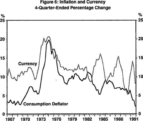
The dynamic forecasts based on extrapolating the behaviour of currency in 1989 (panel 1 of Table 4) perform much better than other indicators because its growth rate happened to be falling sharply at that time. However, if the authorities had been able to forecast the future growth of currency perfectly (panel 2), inflation would have been predicted to fall sharply in 1990 to 3.4 per cent, and then rise to 5.7 per cent by the end of 1991 – essentially reversing the profile of the actual outcome for inflation over this period. The rolling horizon forecasts (panel 3) also perform poorly, with RMSEs well in excess of those obtained by using the simple autoregressive model. This suggests that special factors influencing the behaviour of currency in 1990 and 1991 were so important that it is unlikely to have been very useful for forecasting inflation at the time.
(ii) Broad Money and Credit
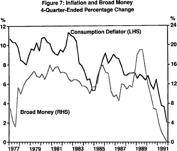
Financial liberalisation and innovation are likely to affect the demand for narrower aggregates more heavily than very broad aggregates. This is because the latter include a much broader range of financial institutions and products, so that switches between individual components in response to financial change have less impact on their overall sum. Broad money has a reasonable leading relationship with major swings in inflation over the full sample period shown in Figure 7. Moreover, its performance since 1983 appears to be better than that for currency. It leads the upturn and fall in inflation from 1985 to 1987 (whereas currency has an inverse pattern), and it leads the deflation of the 1990s (whereas currency clearly lags it). The main exception to this is late 1988 and 1989, when broad money growth accelerated but was not accompanied by increased inflation. This episode corresponds with the elimination of Statutory Reserve Deposits (SRDs), which saw bank funding of their lending activities return to deposits, rather than bill financing, and to Australian dollar, as opposed to foreign liabilities. The sum of coefficients on broad money in equation [2] (see Table 2) is correctly signed and significantly different from zero. As expected, the hypothesis of no structural break over the entire period is rejected. One reason why broad money may have some useful leading information for nominal demand and (hence) inflation pressure, however, is that it is closely linked with the behaviour of credit.
Potential problems with the reliability of monetary aggregates as indicators in liberalised financial markets have led some to suggest that credit may be a superior alternative.[14] While financial liberalisation partly undermined the position of banks as providers of liquid liabilities, depository institutions continue to play an important role in the provision of credit to corporate borrowers. Small and medium-sized companies can find it prohibitively expensive to borrow directly in open equity and securities markets. Similarly, the housing market is primarily financed through borrowing. In liberalised markets, since the early 1980s, credit is likely to have become a better leading indicator of nominal spending and inflation. Unconstrained by regulations, borrowing is more likely to be based on expectations about future income and wealth and on the cost of borrowing influenced by monetary policy. A shift in monetary policy that reduces expectations about future income and wealth, while also increasing the cost of borrowing, affects current decisions about future spending by businesses and households. While causation is from monetary policy to unobservable expected future income, wealth and spending, it should first be observable in reduced credit demand before actual spending and activity (and certainly inflation) is observed to decline.[15]
Credit growth and inflation are shown in Figure 8. Credit clearly leads major turning points in inflation, including the most recent deflation. The only exception to this rule is the late 1980s, when credit growth picked up significantly without any apparent implications for inflation. Its overall usefulness as an indicator within the framework provided by equation [2] appears to be significant, with the sum of coefficients on lags of credit growth being significantly different from zero at the 5 per cent level. As with the monetary aggregates, the hypothesis of no structural change in the coefficients is rejected.
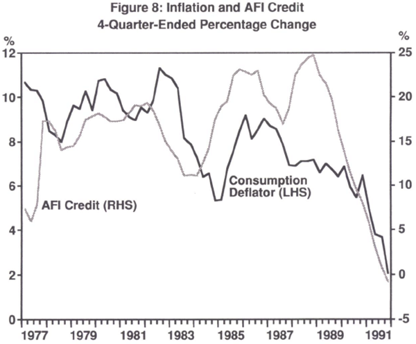
Broad money and credit may have similar leading relationships with inflation because loans are financed out of financial institutions' overall liabilities. To the extent that bank share price developments do not facilitate major capital raising by banks (also a liability that finances loans), broad money is a reasonable proxy for the latter. Lending decisions are made in response to private credit demand related to spending plans. Financial institutions then essentially ‘buy’ the deposits required to finance these demands.[16] Hence major swings in credit and broad money could be useful indicators, though not causes, of private sector spending plans and (later) inflation for similar reasons. In Figures 7 and 8 broad money and credit have a very similar profile, except in the period 1987–88, when credit accelerated earlier than did broad money, and for different reasons.[17] This period corresponds with a sharp jump in bank share prices in response to the introduction of dividend imputation, which greatly favoured bank shares.[18] Banks found it much cheaper to raise new capital in this period.
Dynamic out-of-sample predictions of inflation using forecast values of broad money and credit, which accord some weight to their behaviour in 1989 (panel 1 of Table 4), predict steady inflation in 1990 and 1991. AFI credit performs better than broad money because its growth had already begun to fall somewhat from the end of 1988. The results shown in the second panel suggest that if the impact of monetary policy on broad money and credit growth in 1990 and 1991 could have been foreseen in 1989, both indicators would have performed better than any of the others in predicting the deflation. The RMSEs for these dynamic forecasts are well below that for the naive autoregressive model. This picture is also confirmed with the rolling horizon forecasts, where both indicators predict inflation slightly less than the actual outcome in 1991Q4.
(c) Asset Price Indicators
Nominal asset prices are potentially useful leading indicators because they are driven by expectations about the future. Equity prices, for example, are fundamentally determined by the present discounted value of future dividends. Property prices, in principle, are driven by the present discounted value of future rentals, and so forth. That is, nominal asset prices are theoretically determined by at least two main factors: (a) expectations about future nominal returns, which are principally driven by expectations about activity and inflation, and (b) the discount rate, which is affected by monetary policy. The potential usefulness of asset prices in gauging the stance of monetary policy derives from their interactive nature. Changes in monetary policy affect expectations about future activity, inflation and the rate at which future expected returns are discounted. Asset prices therefore provide feedback information from financial markets concerning their ‘view’ about the likely impact of policy changes. For example, an unanticipated expansionary monetary policy is likely to cause asset prices to jump immediately in real terms, given the inertia of inflation. Increased borrowing and spending in response to lower interest rates would lead to higher real activity and eventually inflation. As activity returned to potential and inflation stabilised, asset prices should be left unchanged in real terms.[19]
If monetary policy was the only factor driving the business cycle and asset prices, this would be reasonably unambiguous information. A sustained tightening that caused asset prices to fall would reflect expectations of a decline in activity and lower goods price inflation in the long run. However, asset price variability may derive from at least two other sources which may have little to do with the stance of monetary policy and likely future inflation:
- changes in real fundamentals: that is, changes in the after-tax real stream of dividends, rents, etc. This could be caused by a wide range of factors including changes in technology and investment; productivity; the profit share, which is influenced by incomes policy; tax treatment of dividends; market deregulation and reforms; world trading arrangements; population change; and
- market inefficiencies: such as ‘feedback’ and ‘noise’ trading, which may lead to both ‘bubble-like’ movements in asset prices unrelated to fundamentals, and increased volatility of asset prices.
Asset price movements as a result of changes in real fundamentals should not lead to sustained inflation or deflation provided monetary policy remains neutral. Such asset price changes may, therefore, represent a permanent relative price shift related to anticipated changes in real wealth. Asset price movements driven by market inefficiencies should normally be transitory – deviating from fundamentals for a time before reverting back again.[20] Such transitory asset price volatility need not be transmitted into sustained spending and inflation cycles, particularly if monetary policy is broadly neutral. However, if such price movements are persistent over a long enough period, it cannot be ruled out that they could be mistakenly attributed to fundamentals and result in some cycle in activity and goods prices.
Figure 9 shows the level of equity prices, house prices and commercial property prices in relation to the level of the consumption deflator using quarterly data from the beginning of the 1970s. In Figure 10 these are aggregated approximately according to their respective nominal quantities. Figure 11 shows the four-quarter-ended percentage changes in the aggregate asset price index and the consumption deflator. As expected, asset prices are much more volatile than the consumption deflator, particularly equity prices. What is most striking about Figures 9 and 10 is the sharp rise in asset prices, led at first by equities, in the second half of the 1980s. While commercial property prices by the end of 1991 appear to have fallen back, the real increase in equities and house prices has been sustained. These seemingly ‘permanent’ relative price shifts are reflected in the aggregate asset price index, which has risen in real terms.
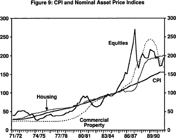
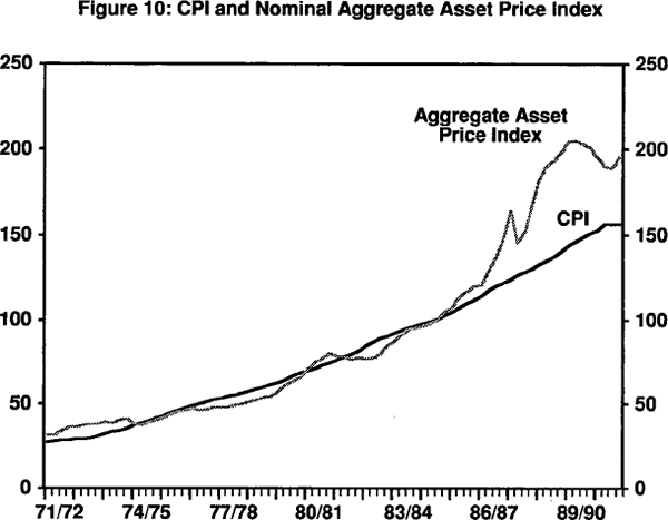
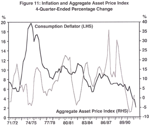
In Figure 11, percentage changes in the aggregate asset price index do not appear to have any consistent leading relationship with goods price inflation. Prior to deregulation the lack of a relationship may be the result of liquidity constraints. These constraints meant that improved asset value could not easily be borrowed against to affect spending on goods. This argument is much less convincing for the 1980s. At least two major peaks in asset price inflation in 1987, due to equities, and in 1988–89, due to property, were not reflected in any pick-up of inflation. Reduced asset price inflation, and deflation in the case of commercial property has, however, led the sharp fall in consumer price inflation in the 1990s. This very mixed pattern is reflected in the estimates presented in Table 2. Neither aggregate asset prices, equity prices, house prices nor commercial property prices were found to be significant leading indicators of inflation in the tests employed here.
(d) The Yield Curve as an Indicator of Inflation Changes
In addition to having indicators of the future level of the inflation rate, it is useful to have indicators of expected changes in its future profile. As discussed above, an increase in inflation generated by some real shock that is not accommodated by monetary policy is likely to be temporary. In such cases inflation would be expected to slow at some future point without a tightening of monetary policy. In contrast, higher inflation caused by a nominal shock may be sustained in the face of no adjustment to monetary policy. An indicator of expected future changes in the path of inflation may help in identifying the nature of the disturbances, and thus aid in the formulation of policy.
The forecasts based on autoregressive predictions of the indicator variables shown in panel 1 of Table 4 performed poorly in predicting future changes in inflation. Only half of the indicator models predicted lower inflation in 1991 than in 1990, and none came close to the actual magnitude of −4.3 percentage points. This situation is improved when actual values of some of the indicators are used (especially for the terms of trade/import price, broad money and credit models). But this would have required very accurate forecasts of the indicators' behaviour in 1990 and 1991. The basic problem with the dynamic forecasts is that, in most cases, forecasting the indicator variables is as difficult as forecasting the inflation rate itself.
The yield curve offers the advantage that it incorporates, in principle, the market's expectation of the future path of inflation. Expected future inflation rates should take into account expectations about all the indicator variables, as well as the underlying causal mechanisms. Using the yield curve thus removes the need to forecast the indicator variables. The slope of the yield curve summarises all available current information about the expected evolution of the inflation rate, and thus might provide superior forecasts of changes in inflation to those provided from the dynamic forecasts reported in Table 4.
The rationale for using the slope of the yield curve as an indicator of changes in the path of inflation comes from the standard Fisher equation:
where Et denotes the expectation at time t,
 the inflation
rate between time t and m,
 the nominal m-period
interest rate at time t and
 the real m-period
interest rate at time t.
The observed rate of inflation equals the expected rate plus a forecast error:
Substituting [4] into [3] gives:
To obtain a relationship between the slope of the yield curve and the change in the inflation rate, the n-period inflation rate is subtracted from [5] yielding:
This shows that the slope of the nominal yield curve between securities of length
m and n should provide unbiased forecasts of the difference in the inflation
rate between today and time m and the inflation rate between today and time
n, provided two assumptions are made. These assumptions are that expectations
are rational and incorporate all available information, and that the slope
of the real yield curve
 is constant.
However, the assumption of a constant real yield spread is a strong one. In
fact, changes in real interest rates are a key element of the monetary policy
transmission mechanism when expectations of inflation are partly
backward-looking. In addition, there is considerable empirical evidence
rejecting the restrictions implied by constant real interest rate
spreads.[21]
The fact that the slope of the real yield curve changes through time implies that changes in the slope of the nominal yield curve do not solely reflect changes in inflation expectations. Thus, Frankel and Lown (1991) argue that the yield gap between a long-maturity instrument and a short-maturity instrument should provide superior forecasts of the change in inflation than those generated by the spread between securities which exactly match the period over which inflation is being forecasted. They present evidence using US data in support of this view, while Lowe (1992) presents similar evidence for Australia.
The empirical work on the predictive power of the yield curve using data from a wide range of countries has typically found that the slope of the yield curve (regardless of horizons used) provides little information concerning the change in inflation between periods that are shorter than one year. The results for Australia are no exception. However, Mishkin has shown that the slope of the yield curve does well in forecasting changes in inflation over periods longer than one year.
The principal focus of the results presented below is on the ability of the yield curve to predict the difference in the inflation rate between today and one year in the future, and today and two years in the future. The two year/one year comparison is a useful one for policy. Monetary policy typically operates with a lag so that actions today have little effect on today's inflation rate. While the exact length of the lag is uncertain, monetary policy changes are thought to have their maximum impact on real activity, and hence prices, at least one year after the policy change is made. Given this lag, it is useful for the monetary authorities to have an indicator of not only the inflation rate over the next year, but also an indicator of inflationary pressures in the following year, for this is where the impact of policy might reasonably be expected to be most acutely felt.
Since the consumption deflator measures average prices over the quarter, and not prices at the end of the quarter, the average of the quarter's three end-month interest rates is used in calculating the slope of the yield curve. The sample period runs from September 1982 to December 1991. The commencement date is chosen to coincide with the change from the tap to the tender system for the issuing of government bonds. The 10-year bond/180-day bank bill spread is used as our measure of the slope of the yield curve. Thus, the equation to be estimated is:
Estimation is Ordinary Least Squares and the Newey-West standard errors have been used. The results for selected forecast periods are reported in Table 5.
 |
 |
||
|---|---|---|---|
| α | β |
 |
|
 |
−0.08 (0.15) |
0.03 (0.07) |
−0.02 |
 |
−0.09 (0.20) |
0.02 (0.06) |
−0.04 |
 |
−0.07 (0.26) |
0.30 (0.08) |
0.24 |
 |
0.02 (0.12) |
0.28 (0.05) |
0.50 |
| Note: m and n are expressed in terms of months. | |||
The results show that the slope of the yield curve provides no information concerning
the difference in the inflation rate over the subsequent six months and the
inflation rate over the next twelve months. The same is true for the difference
in the inflation rate over the next three months and the rate over the next
six months. These results confirm that the yield curve has no information concerning
the short-run evolution of inflation. In contrast, over slightly longer periods
the yield curve does provide considerable information on the evolution of inflation.
The
 for the equation explaining the difference
in the inflation rate over the next two years and the inflation rate over the
next one year is 0.50. In contrast, the
 statistics from the shorter horizon regressions
are less than zero. The results also suggest that the yield curve is useful
in predicting the relative inflation rates over the next six months and two
years, although the parameters are estimated less precisely than over the longer
period.
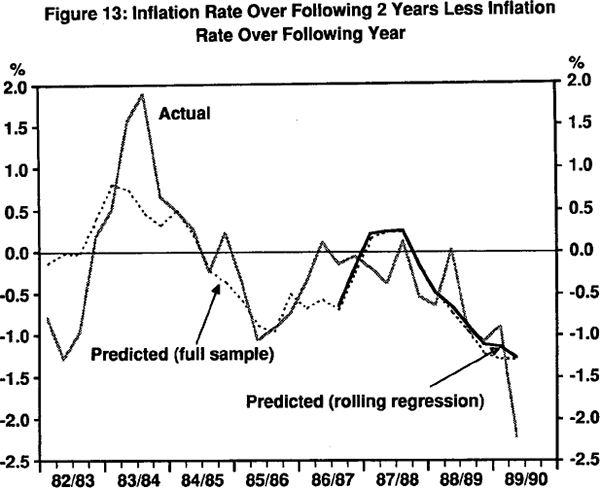
Given the policy interest in predicting the difference in the inflation rate over the next two years and the rate over the next one year, we now turn to a closer examination of the yield curve's ability to predict this difference. Figure 12 shows the slope of the yield curve and the inflation rates which actually occurred over the following one and two years. It shows the strong correlation between the slope of the yield curve and changes in the rate of inflation; periods characterised by a negatively (positively) sloped yield curve are typically followed by a decline (increase) in the rate of inflation. The one exception is the positively-sloped yield curve in the second half of 1987 and early 1988. In this case the predicted increase in inflation did not eventuate (as with the output gap and credit indicators). However, when one examines the CPI inflation rate it does show an increase in inflation along the lines suggested by the slope of the yield curve. This difference in the results comes from the inclusion of mortgage interest rates in the CPI. This raises an interesting question. That is, when key price indices are behaving differently, which inflation rate is the market incorporating into the yield curve? This issue goes beyond the scope of this paper, but is potentially important when the headline inflation rate differs from other key inflation rates.
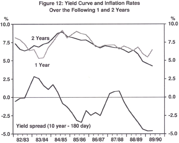
Figure 13 presents the actual and predicted differences in the inflation rate over the next two years and the inflation rate over the next one year. Two predictions of the difference are shown from the first quarter of 1987. The first uses the entire sample to estimate equation [7] and calculate the predicted difference. The second uses rolling regressions, so that only information actually available at the time the forecast would have been made is used in making these static forecasts. The two sets of predictions are essentially identical. The figure shows that while the curve has not predicted all future changes in the inflation rate, it has correctly forecast a number of the major turning points. In particular, at the end of 1989 the yield curve was predicting a significantly lower rate of inflation in 1991 than in 1990. While it failed to predict the full extent of the slowdown in inflation, it performed better than most of the other indicators considered in this study. This can be seen in Table 6. The yield curve certainly outperforms the dynamic predictions based on autoregressive forecasts of the indicator variables. It also performs better than those based on actual values of the indicators, though not much better than the forecasts based on the terms of trade and import prices, broad money, and credit.
| Using AR forecasts of indicators |
Using actual values of indicators |
||
|---|---|---|---|
| Autoregressive | −0.3 | −0.3 | |
| Output gap | −0.5 | −0.2 | |
| Wages | +1.1 | +0.1 | |
| Terms of Trade (TOT) | −0.4 | −1.3 | |
| TOT and Import Prices | −0.1 | −1.7 | |
| Currency | +0.4 | +2.3 | |
| Broad Money | 0.0 | −2.2 | |
| AH Credit | +0.1 | −1.7 | |
| Dynamic Forecasting Models (obtained by subtracting 1990Q4 forecast from 1991Q4 forecast) | |||
4. Interpreting the Recent Unusual Behaviour of Some Indicators
Most, though not all, of the indicators analysed earlier proved to possess some information useful for forecasting inflation, in addition to that contained in lagged inflation. However, in the past few years the behaviour of some of these indicators appears to have been at odds with subsequent inflation experience. Most of the indicators predicted an acceleration of inflation from 1988 to early 1990. Inflation, however, continued to decline moderately over this period. Subsequently, only some of the indicators predicted a fall in inflation. None predicted the full extent to which inflation declined during 1991.
(a) Demand Pressure and Wage Restraint in the Late 1980s
Over earlier periods, past inflation and the output gap, in particular, were reasonably reliable leading indicators. Estimated to the late 1980s, this equation was unique in having parameters that were both statistically significant and structurally stable. From 1988 to 1990, however, a large positive output gap was not reflected in any acceleration of inflation. Structural instability appears to have become a problem with the equation at this time. Similarly, rapidly growing credit and broad money, a strong terms of trade and the asset price boom all suggested ex ante inflation pressure that was not actually realised. This apparent breakdown in the relationship between leading indicators and inflation in the late 1980s can be reconciled with the view of the transmission mechanism set out in section 2, provided some attention is paid to the role of incomes policy under the Accord in this period.
It was argued earlier that wage-tax trade-offs via the Accord contained the ex ante wage pressure implied by the strength of the economy and the terms of trade from 1988 to early 1990. This restraint in the face of strong growth in nominal demand was bound to shift demand pressures to other parts of the economy. In particular, there was a strong increase in real profits (Figure 14), and this contributed to the asset price inflation already in progress at the time. Empirical evidence of a link between asset prices, profits and the interest rate is set out in Appendix B.
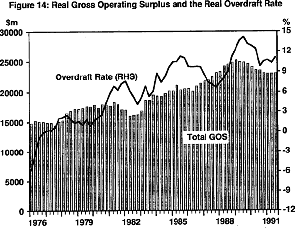
In addition to rising nominal demand and the wage restraint/profit mechanism, there was also undoubtedly an additional speculative element in rising asset prices, as investors anticipated continuing capital gains. This speculation was also facilitated by favourable expectations unfolding in the context of newly-liberalised financial markets.[22] While the share market overshot in this respect in 1987, possibly due to events occurring on foreign stock exchanges, equity prices were still high relative to goods prices in 1988 and 1989 (Figure 9). Furthermore, commercial property and house prices also rose steeply in these later years.
The strong profit performance in the late 1980s also contributed to the strength of real activity. Business expectations about future returns were favourable, so that actual and intended fixed investment grew rapidly at this time. Investment plans and a preference for debt financing also contributed to the observed sharp rise in credit. The other major factor influencing the behaviour of credit was the inflation of asset prices itself. On the supply side, this greatly increased the collateral available to banks and other financial institutions. On the demand side, asset price inflation contributed to gearing for speculative purposes, as investors anticipated future capital gains.
Thus, by containing wages in the face of strong nominal demand, the Accord made it difficult to interpret the behaviour of the standard indicators. The upswing in activity, rising nominal wealth, strong credit growth, and the improved terms of trade risked spilling over into increased inflation.[23] While the Accord process could delay the impact of such ex ante pressure on wages for some time, it could not do so indefinitely. Tax cuts in exchange for wage restraint, for example, cannot be repeated often, given the budget deficit constraint. The Accord therefore broke temporarily the nexus between the output gap and inflation. This nexus could not, however, be broken permanently if nominal demand continued to rise at an unsustainable rate. If monetary policy had not been tightened, ex ante wage and price pressures would have led to an increase in observed inflation.
(b) Deflation and Indicators in the Early 1990s
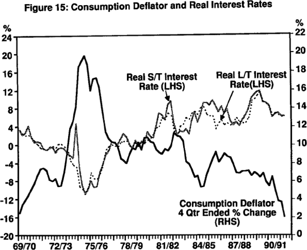
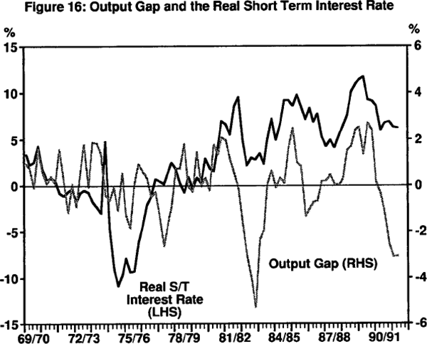
Monetary policy was tightened from early 1988, as reflected in the behaviour of the real interest rate shown in Figures 15 and 16. The earliest signs that changes in interest rates had succeeded in shifting private sector expectations to the point where inflation would begin to decline, were provided by those indicators most closely associated with the monetary transmission mechanism:
- the strength of the exchange rate in the late 1980s and its subsequent steadiness in the face of the declining terms of trade from early 1990;
- the sharp decline in the growth of credit (and broad money); and
- the inverted yield curve.
In addition, while they appear technically to have had little information useful for forecasting inflation, asset prices declined well ahead of the disinflation.
The role of the relatively firm exchange rate, in the face of a declining terms of trade, as a leading indicator of the fall in inflation was analysed in some detail in section 3, and requires little further elaboration here. Other important aspects of the transmission mechanism do require some discussion. First, why did asset prices lead the downswing in activity and inflation, yet appeared to have little information for forecasting inflation in the simple temporal ordering tests conducted in section 3? Second, earlier work has shown that credit typically lags the cycle in GDP in Australia.[24] Such a finding is inconsistent with the key transmission mechanism of intertemporal substitution discussed in Section 2.
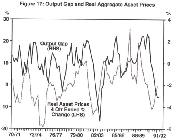
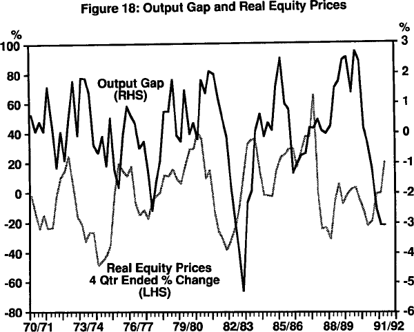
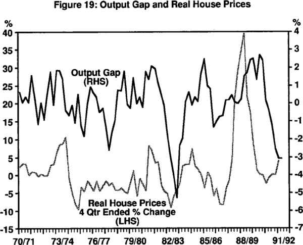
With regard to asset prices, Figures 17, 18 and 19 compare aggregate real asset prices, real equity prices and real house prices, respectively, with the output gap. Here the leading relationship is relatively unambiguous. This is consistent with the role of asset prices in influencing spending and activity via real wealth effects.[25] Since the lead time appears quite long (about one year for the aggregate asset price series), and activity itself affects inflation with a relatively long lag, it is not surprising that asset prices were insignificant in the equation [2] tests based on six lags. More importantly, the very strength of asset price inflation in the late 1980s, which must dominate the reported empirical results, was directly linked to the role of the Accord in containing wage and price inflation. The failure of inflation to accelerate contributed to the extreme movement in asset prices. The link between activity and asset prices was not so distorted, so the relationship between them is clearer. The consistency of their behaviour with the monetary transmission mechanism during the disinflation phase suggests that asset prices should certainly not be ignored in the future.
The indicator role of credit since financial deregulation has been re-examined by Blundell-Wignall and Gizycki (1992), using more recent data than that available to Bullock, Morris and Stevens. This more recent study suggests that if the sample period excludes data from the regulated period and is extended to 1991Q4 (compared to 1987 in the earlier study), then:[26]
- business credit unambiguously leads business fixed investment;
- total credit adjusts endogenously to prior movements in the level of the loan rate and nominal GDP; and
- GDP also adjusts to prior movements in the level of the loan rate and credit.
Since the loan rate is weakly exogenous in these tests (does not adjust to prior movements in GDP and credit), the results are consistent with the assumptions of intertemporal substitution. Monetary policy impacts on the loan rate causing agents to delay spending plans and reduce current borrowing. This mechanism appears to have been at least partly responsible for the slowdown in credit growth prior to the most recent slowing in the economy. The effect on credit has some useful information for forecasting subsequent changes in investment and GDP.
It is still too early to conclude that these results will prove robust for future turning points, and the evidence suggests that two-way causation is also present. However, it is interesting to note that similar findings concerning the improved indicator qualities of credit have been found for the U.S. economy.[27] A possible reason for this is that in regulated financial markets, which include the presence of deposit rate ceilings, financial intermediaries cannot readily finance any demand for credit based on private sector plans for future expenditure. Instead, the bulk of lending is financed from ‘core’ deposits. Banks are unable to bid directly for funds, and must depend upon growth in private sector saving to fund the demand for loans. Since private saving is positively related to income, movements in GDP are more likely to precede movements in loans financed from ‘core’ deposits during periods affected by financial regulations. In a liberalised financial system institutions can respond more quickly to loan demand based on future spending plans. They manage their liabilities, simply buying any additional deposits they need to finance this lending in wholesales markets.
However, while those indicators most consistent with the transmission of monetary policy in liberalised financial markets predicted part of the slowing of inflation from the end of the 1980s, they failed to predict the full extent of its decline. Since most of the indicators focused upon in this period are conditioned by forward-looking expectations, this raises the question of why markets appear to have underestimated the decline.
There are two main possibilities. First, given the stance of monetary policy, there may have been unexpected real shocks which acted to reduce inflation. The extent of the decline in the terms of trade after the end of the 1980s is one such possibility. However, the fact that the lower terms of trade was not associated with a fall in the exchange rate, suggests a more important reason for the failure of the forward-looking indicators to predict the decline in inflation. The reason is that the market did not predict the extent to which the authorities would pursue a tight monetary policy in order to ensure a low-inflation outcome. This interpretation would be consistent with the delay in the adjustment of economic activity, and some of the other indicators such as credit, during the late 1980s.
5. Concluding Remarks
It was argued that leading indicators are extremely important for conducting monetary policy in a pre-emptive fashion. A range of indicators were analysed using various statistical tests, and their out-of-sample forecasting properties during the recent period of disinflation were explored. By and large those indicators found to be most useful were consistent with a view of the economy in which there is a pro-cyclical component to inflation and considerable inertia in price expectations, and where monetary policy is transmitted via intertemporal substitution and changes in the exchange rate and wealth.
In addition, two special features of the Australian economy could not be ignored when interpreting the otherwise standard range of indicators. First, as a commodity-exporting country, the largely exogenous terms of trade was found to be important. The interaction between the terms of trade, the exchange rate and the stance of monetary policy was of particular interest in this respect. The second factor was the use of incomes policy via the Accord during the 1980s and early 1990s. In the face of strong ex ante inflation pressure, the Accord contained wages and prices. This containment, however, contributed to increased volatility in other areas of the economy. In particular, it affected the behaviour of a range of indicators used in assessing the stance of monetary policy. Thus, not only do a range of leading indicators need to be continually assessed in the pre-emptive setting of monetary policy, but any period-specific effects caused by special factors also need to be taken into account.
With regard to the future conduct of monetary policy during the 1990s, monitoring and assessing the level of economic activity in relation to potential output and the most recent momentum in inflation are likely to remain important considerations. But it is also worth emphasising again that in an economy with deregulated financial markets the transmission of monetary policy depends heavily on wealth and intertemporal substitution effects. This has important implications for the selection of indicators. In particular, credit growth, asset prices and the yield curve need to be considered as potentially important leading indicators. In addition, the volatile nature of the price of Australia's commodity exports make it essential also to consider the behaviour of the exchange rate in conjunction with movements in the terms of trade. While short-run movements in any one of these indicators will always need to be treated with caution, it seems unlikely that new trends in nominal demand and inflation could behave independently from all of them over long periods of time.
Appendix A: Data
All data is sampled quarterly and, where appropriate, is seasonally adjusted. Subject to availability, data is collected for the period from March 1966 to December 1991. The consumption deflator is consistently applied to obtain real series based in 1984/85.
Three asset price indices, based in 1984/85, are recorded. The All Ordinaries nominal share price index, available from September 1969, is obtained from Data Express. Callen (1991) provided a weighted average of median established dwelling prices and estimates of commercial property prices for the period March 1990 to September 1991. An historical house price index, obtained from the ABS, combines data from the Real Estate Institute of Australia and earlier Valuer-General's Department statistics back to March 1968. This series was spliced onto the more recent data from Callen (1991). Similarly, nominal commercial property prices for the Sydney CBD were obtained from internal sources back to March 1968 and spliced onto Callen's 1980s data. An aggregate asset price index was constructed from these three asset classes. The weights attributed to the share, housing and commercial property price indices were 29 per cent, 59 per cent and 12 per cent, respectively.
Broad money and all financial intermediaries credit statistics, only available from March 1976, were provided by the Economic Analysis Department of the Reserve Bank of Australia (RBA), along with currency, real gross domestic product, the consumer price index and the consumption deflator. All interest rates were obtained from the RBA Bulletin. The 90 and 180 bank bill rates are from Table F. 1, the 10-year bond rate is from Table F.2 and the loan rate on overdrafts of $100,000 and over (maximum) is from Table F.3.
A wage rate series was constructed from March 1969 as the ratio of average earnings of non-farm wage and salary earners ($/week) to average weekly hours of wage and salary earners. These series were sourced from the Activity Section, Economic Analysis Department, RBA and the Commonwealth Treasury's NIF-1 OS model database published in ABS catalogue No. 1340.0, respectively.
Appendix B: Asset Prices, Profits and the Interest Rate
Asset price inflation in the late 1980s has been the focus of such attention that the influence of profits is worth spelling out. While other speculative factors were also important, it is nevertheless the case that for a given level of interest rates increased profits are the key ‘fundamentals’ factor driving asset prices. For example, if q is the value of the stock market, then the return on holding shares is the expected rate of change of the value of the stock market plus the expected dividend return. Arbitrage between short-term bonds and shares therefore implies:
where i is the bond rate and π is profits. Since in the steady-state the expected change in the value of the stock market is zero, a long-run equilibrium relationship is implied between the value of the share market, profits and the interest rate (i.e. q = π/i). Similar propositions apply to all other asset prices.
The empirical importance of this mechanism for Australia is demonstrated in Table B1, which shows the results of cointegration tests for such long-run relationships for both share prices and the aggregate asset price index. The results suggest that both of these series are cointegrated with profits and the interest rate, with the expected signs. Also shown in the table are the error correction coefficients for the adjustment of asset prices consequent upon prior movements in profits and interest rates. These also have the expected signs, and are significantly different from zero at the 1 per cent level. For the purposes of illustrating the importance of the Accord and profits in the late 1980s, these latter results are important. This is because the error-correction results imply causation. Asset prices adjust endogenously to the weakly exogenous profit and interest rate variables.
| Long-run coefficients |
ADF statistics | Error correction coefficients |
|
|---|---|---|---|
| (Sample: 1969Q3–1991Q4) | |||
| Nominal share price | |||
| nominal profit (GOS) | 0.952 |
 −2.437** −2.437** |
−0.147 (−2.37) |
| nominal interest rate | −0.699 | ||
| (Sample: 1969Q3–1991Q3) | |||
| Nominal aggregate asset price | |||
| nominal profit (GOS) | 0.832 |
 −2.934** −2.934** |
−0.145 (−3.57) |
| nominal interest rate | −0.188 | ||
| Note: Augmented Dickey-Fuller tests (with the null of
a unit root and, therefore, no cointegration) are performed
on each model using the following methodology. La Grange
multiplier tests are used to determine the lag length
in each of the residuals equations (which initially
include both a trend and drift term) sufficient to account
for all serial correlation. Here, the lag length is
initially set to 4 but decreased if the LM test does
not reject the null of no autocorrelation. Then: (i) Test the significance of the TREND term. If it is significant, test the null hypothesis against N(0, I) critical value; otherwise, test the null hypothesis against the Dickey Fuller (1976) table of critical values,  . .(ii) If the null is accepted and the trend term is insignificant, drop the trend, re-estimate the equation and test the significance of the DRIFT term. If it is significant, test the null hypothesis against N(0, I) critical value; otherwise, test the null hypothesis against the Dickey Fuller (1976) table of critical values,  . .(iii) If the null is accepted and the drift term is insignificant, drop the drift, re-estimate the equation and test the null against the Dickey Fuller (1976) table of critical values,  . .Here: ** the null of no cointegration can be rejected at the 5 per cent significance level; * the null of no cointegration can be rejected at the 10 per cent significance level. |
|||
Footnotes
Authors are, respectively, Head of Economic Research Department, Senior Research Economist and Assistant Research Economist. [*]
See Bullock, Morris and Stevens (1989) and Stevens and Thorp (1988). One recent foreign example includes Switzerland, where a serious inflation episode resulted from reliance on money base targeting in the face of (unpredicted) technological changes that reduced the demand for base money in the late 1980s. [1]
See Blundell-Wignall, Browne and Manasse (1990) for a summary of a recent study by the OECD. [2]
The theoretical model is set out in Blundell-Wignall and Gregory (1990) along with empirical evidence. Some historical episodes are discussed at length in Stevens (1992). [3]
Here it is also helpful if the data series is not subject to major revisions, is promptly available and is reported at a reasonably high frequency. [4]
The money base was also tested. Interestingly, currency outperformed this variable as an indicator in all respects. Consequently, only the results for currency are reported in the results below. [5]
This is a very standard approach to the analysis of indicators used in virtually all studies in this area. A recent example is Hallman, Porter and Small (1991). [6]
See, for example, Lucas (1977), Hodrick and Prescott (1980), Danthine and Girardin (1989) and Kydland and Prescott (1990). [7]
One possible explanation for this is that the Hodrick-Prescott measure of potential output may be excessively influenced by the most recent recession. If this were true, more of the increase in activity in the late 1980s would be due to improved ‘fundamentals’ or trend growth, so that the inflationary gap is exaggerated in this period. However, doubling the value of λ to 3200 (making the trend more linear) does not eliminate this gap – nor does it greatly affect the estimation results. [8]
See Reserve Bank Annual Reports in 1989 and 1990 for a discussion of these perceived pressures. [9]
This is consistent with earlier work on this topic in Australia. For example, Fahrer and Myatt (1991). [10]
The empirical relevance of such wage-tax trade-offs in a bargaining model of wage determination in Australia has been demonstrated elsewhere. See Blundell-Wignall and Stevens (1991). [11]
The nominal and real exchange rates should adjust endogenously to major swings in the exogenous terms of trade. This is set out theoretically in Blundell-Wignall and Gregory (1989), where empirical support for this proposition is also presented. See also Gruen and Wilkinson (1991) for more recent evidence. [12]
Currency demand also rose in the mid-1980s with the use of the $100 note, and may have been related to taxation considerations. [13]
King (1986), Friedman (1983), and Bernanke and Blinder (1988). [14]
This is tested formally in Blundell-Wignall and Gizycki (1992), the results of this study being referred to in more detail below. [15]
Correspondingly, higher cost wholesale instruments such as CDs and bills have been used increasingly to finance lending, in addition to banks' traditional deposits. [16]
The SRD explanation for the acceleration in broad money does not explain the behaviour of credit, which is more likely to be explained by underlying demand factors. [17]
This is because banks' profits are fully taxed. This is tested and discussed at greater length in Blundell-Wignall and Gizycki (1992). [18]
See a theoretical treatment of these dynamics in Blanchard (1981). [19]
Cutler, Poterba and Summers (1990) examined data from thirteen countries, covering equity and bond markets, house prices, collectables, gold and exchange rates over relatively long sample periods. They found that there were excess returns available in these markets which were positively serially correlated at high frequency and negatively correlated at longer horizons. These patterns emerged repeatedly in their samples, and their pervasive nature was taken to imply that they were inherent features of the speculative process. That is, over short horizons asset prices were driven by their recent past behaviour, but there is reversion to ‘fundamentals’ in the longer run. [20]
See Mishkin (1991). [21]
This is argued, for example, in Macfarlane (1991). [22]
The unsustainability of this process was discussed at the time by Macfarlane (1989). [23]
See Bullock, Morris and Stevens (1989). [24]
Here it is worth noting that temporal ordering tests along the lines of equation [2], but with output on the left-hand side, show asset prices to be relatively useful leading indicators of the output gap. [25]
Specifically, the sample period is 1984Q1 to 1991Q4. Error correction methods are used to test causality between GDP, credit and the loan rate. While two-way causation is present in the relationship between GDP and credit, this was not the case for business credit and investment. Business credit unambiguously leads investment. [26]
Thus Bernanke and Blinder (1988) found that credit had a much more reliable relationship with economic activity in the 1979 to 1985 period compared to money than during 1974 to 1979, when money had a better relationship. O'Brien and Browne (1992), in a recent OECD study, show that the leading indicator properties of credit in the United States greatly improved over the 1983Q1 to 1991Q2 period, compared to an earlier sample period of 1970Q1 to 1982Q4. [27]
References
Andersen, P.S. (1992), ‘OECD Country Experiences with Disinflation’, this volume.
Ball, L. (1990), ‘Credible Disinflation with Staggered Price Setting’, NBER Working Paper No. 3555.
Bernanke, B.S. and A.S. Blinder (1988), ‘Credit, Money and Aggregate Demand’, American Economic Review, Papers and Proceedings, 78, pp. 435–439.
Blanchard, O. (1981), ‘Output, the Stock Market, and Interest Rates’, American Economic Review, 71, pp. 132–143.
Blundell-Wignall, A., F. Browne and P. Manasse (1990), ‘Monetary Policy in Liberalised Financial Markets’, OECD Economic Studies, No. 15, pp. 145–178.
Blundell-Wignall, A. and M. Gizycki (1992), ‘Credit Supply and Demand and the Australian Economy’, Reserve Bank of Australia Research Discussion Paper 9208.
Blundell-Wignall, A. and R.G. Gregory (1990), ‘Exchange Rate Policy in Advanced Commodity Exporting Countries: The Case of Australia and New Zealand’, in V. Argy and P. de Grauwe (eds), Choosing an Exchange Rate Regime: The Challenge for Smaller Industrial Countries, International Monetary Fund, Washington DC.
Blundell-Wignall, A. and G. Stevens (1992), ‘Fiscal Policy in Australia: Recent Developments and Current Issues’, in Current Issues in Fiscal Policy and Their Implications for the Conduct of Monetary Policy, Bank for International Settlements, Basle.
Bullock, M., D. Morris and G. Stevens (1989), ‘The Relationship Between Financial Indicators and Economic Activity: 1968–1987’, in I.J. Macfarlane and G. Stevens (eds), Studies in Money and Credit, Reserve Bank of Australia, Sydney.
Callen, T. (1991), ‘Estimates of Private Sector Wealth’, Reserve Bank of Australia Research Discussion Paper 9109.
Cutler, D.M., J. Poterba and L. Summers (1990), ‘Speculative Dynamics’, NBER Working Paper No. 3242.
Danthine, J.P. and M. Girardin (1989), ‘Business Cycles in Switzerland’, European Economic Review, 33, pp. 31–50.
Fahrer, J. and J. Myatt (1991), ‘Inflation in Australia: Causes, Inertia and Policy’, Reserve Bank of Australia Research Discussion Paper 9105.
Frankel, J.A. and C.S. Lown (1991), ‘An Indicator of Future Inflation Extracted from the Sleepness of the Interest Rate Yield Curve Along Its Entire Length’, NBER Working Paper No. 3751.
Friedman, C. (1990), ‘Monetary Policy in the 1990s: Lessons and Challenges’, in Monetary Policy Issues in the 1990s, A Symposium sponsored by the Federal Reserve Bank of Kansas City, Wyoming, Aug 30–Sept 1.
Gruen, D. and J. Wilkinson (1991), ‘Australia's Real Exchange Rate – Is It Explained by the Terms of Trade or by Real Interest Differentials?’, Reserve Bank of Australia Research Discussion Paper 9108.
Hallman, J.J., R.D. Porter and D.H. Small (1991), ‘Is the Price Level Tied to the M2 Monetary Aggregate in the Long Run’, American Economic Review, 81, pp. 841–858.
Hodrick, R.J. and E.C. Prescott (1980), ‘Postwar US Business Cycles: An Empirical Investigation’, Carnegie Mellon University Discussion Paper No. 451.
King, S.R. (1986), ‘Monetary Transmission Through Bank Loans or Bank Liabilities?’, Journal of Money, Credit and Banking, 18, pp. 290–303.
Kydland, F.E. and E.C. Prescott (1990), ‘Business Cycles: Real Facts and A Monetary Myth’, Federal Reserve Bank of Minneapolis Quarterly Review, No. 14, Spring, pp. 3–18.
Lowe, P. (1992), ‘The Term Structure of Interest Rates, Real Activity and Inflation’, Reserve Bank of Australia Research Discussion Paper 9204.
Lucas, R.E. (1977), ‘Understanding Business Cycles’, in K. Brunner and A.H. Meltzer (eds), Stabilization of the Domestic and International Economy, North Holland, Amsterdam.
Macfarlane, I.J. (1989), ‘Money, Credit and the Demand for Debt’, Reserve Bank of Australia Bulletin, May, pp. 21–31.
Macfarlane, I.J. (1991), ‘The Lessons for Monetary Policy’, in I.J. Macfarlane (ed), The Deregulation of Financial Intermediaries, Reserve Bank of Australia, Sydney.
Mishkin, F. (1991), ‘Is the Fisher Effect for Real?: A Re-examination of the Relationship Between Inflation and Interest Rates’, NBER Working Paper No. 3632.
O'Brien, P.F. and F.X. Browne (1992), ‘A Credit Crunch? The Recent Slowdown in Bank Lending and its Implications for Monetary Policy’, OECD Working Paper No. 107.
Stevens, G. (1992), ‘Inflation and Disinflation in Australia’, this volume.
Stevens, G. and S. Thorp (1989), ‘The Relationship Between Financial Indicators and Economic Activity: Some Further Evidence’, in I.J. Macfarlane and G. Stevens (eds), Studies in Money and Credit, Reserve Bank of Australia, Sydney.
Taylor, J. (1979), ‘Staggered Wage Setting in a Macro Model’, American Economic Review, 69, pp. 108–113.


