RBA Annual Conference – 2002 G-20 Comparisons of Incomes and Prices: What can we Learn from the International Comparison Program? Steve Dowrick
1. Introduction
The International Comparison Program (ICP) is one of the largest economic and statistical exercises that has ever been carried out. Detailed price surveys have been carried out every five years or so, using standardised methods, enabling the calculation of the real quantities of goods and services that are purchased in each economy. A wealth of information has been generated on the price and quantity structures of the participating countries, enabling international comparisons of the effects of trade policy and other policies on the allocation of resources. A review of the Program was carried out by Kravis and Lipsey (1991). In his paper in this volume, Peter Harper details recent developments and plans.
Probably the best-known feature of the ICP has been the derivation of real output (GDP per capita) measured at purchasing power parity (PPP). This allows comparisons of the real value of production of each country, using a standardised measuring rod. Dividing real production by population yields real GDP per capita, a measure of the level of economic activity and average real domestic income. These PPP-adjusted measures have been used by policy analysts and academic researchers to investigate the efficacy of policies and institutions in promoting economic growth. They are also used by international organisations to compare living standards and to determine the capacity of member countries to benefit from, or contribute to, collective programs such as international aid. The European Community, for example, has used PPP-adjusted income comparisons to determine eligibility for its regional development programs.[1]
In this paper I give examples of the use of ICP data to compare the prices of individual commodities and to compare aggregates such as GDP across the countries that comprise the G-20. I highlight some of the problems that arise with a commonly used method of aggregation, and explain an alternative method. I also demonstrate the value of the ICP in measuring important indicators and predictors of economic development such as the relative prices of investment and consumption goods.
2. Foreign Exchange and Purchasing Power Parity Comparisons of Living Standards
It is well-known that the use of market exchange rates to translate international incomes into a common currency introduces a ‘traded-sector bias’ in comparisons of economic living standards. Whilst exchange rates tend to equate purchasing power over traded goods and services, much of economic production is for domestic consumption only. Wide variations across countries in the prices of non-traded goods and services are not reflected in the market for foreign exchange (FX). So exchange rate income conversions do not reflect the relative purchasing power of consumers in their own countries. Indeed, the Balassa-Samuelson argument[2] suggests that FX income comparisons tend to exaggerate international income differentials by ignoring the lower cost of living that is typically observed in poorer economies, due to cheaper labour-intensive services in the non-traded sector.[3]
The International Comparison Program (ICP) has conducted a series of detailed and standardised price surveys across many countries. The surveyed prices are often expressed as purchasing power parities for commodities (ppp) – the notional rates of exchange between the currencies that would equalise the prices in a common currency. I use lower-case ‘ppp’ to distinguish these commodity-level prices from the aggregate ‘PPP’ which measures the purchasing power of the currency over all the commodities that constitute gross domestic product.[4] The individual ppp's vary considerably according to which commodity is under consideration.
Take, for example, the local currency prices for domestic services and for passenger cars in a sample of nine countries from the 1980 ICP Survey. These prices are listed in the first two rows of Table 1. Local prices are expressed relative to the US dollar. For example, the number in the top left corner of the table indicates that in order to purchase the quantity of domestic services that cost one dollar in the US, a Brazilian would have to spend 19.2 cruzeiros.[5] In other words, the ppp of the Brazilian cruzeiro over domestic services was 19.2 cruzeiros per dollar. The actual 1980 exchange rate was, however, 52.7 cruzeiros per dollar, implying that domestic services in Brazil were relatively cheap, just over one-third of the US price at the prevailing market exchange rate.
| Brazil | Canada | Germany | India | Indonesia | Italy | Japan | South Korea |
UK | |
|---|---|---|---|---|---|---|---|---|---|
| Local currency prices (ppp) | |||||||||
| Domestic services | 19.2 | 3.6 | 8.1 | 1.1 | 177 | 2,103 | 499 | 291 | 1.5 |
| Passenger cars | 19.7 | 0.9 | 1.8 | 13.0 | 597 | 980 | 136 | 546 | 0.6 |
| Exchange rate(a) | 52.7 | 1.2 | 1.8 | 7.9 | 627 | 857 | 227 | 607 | 0.4 |
| US dollar prices(b) | |||||||||
| Domestic services | 0.37 | 3.09 | 4.45 | 0.14 | 0.28 | 2.46 | 2.20 | 0.48 | 3.46 |
| Passenger cars | 0.37 | 0.76 | 0.97 | 1.65 | 0.95 | 1.14 | 0.60 | 0.90 | 1.35 |
| (a) The exchange rate is the average for the year, expressed in terms of
local currency units per US dollar. (b) The US dollar price is the local currency price divided by the exchange rate with the US dollar. US prices are all set at unity. |
|||||||||
These relative prices, translated into US dollars at the prevailing exchange rate, are listed in the fourth and fifth rows of Table 1.
There are several significant points that this table illustrates. First, that the relative prices of non-traded services vary by a huge amount across countries: from a low of 0.14 in India to a high of 4.45 in Germany. We can see that the price of services is consistently high in the richer industrialised countries, where wage levels are high. On the other hand, the relative price of cars, a traded good, does not vary nearly so much across countries.
Second, we can see how the use of market rates of exchange can give a very misleading picture of relative living standards. According to the 1980 ICP Survey, the average income (or GDP) per Brazilian was 109,000 cruzeiros, whilst the average per American was US$11,500. Using the market exchange rate of 52.7 cruzeiros per dollar implies that the average Brazilian income was equivalent to US$2,068, just 18 per cent of US income. But this ignores the fact that domestic services and cars were much cheaper in Brazil than in the US. Using the average of the two reported ppp's for commodities, 19.5 cruzeiros per dollar, suggests that the purchasing power of the average Brazilian income was in fact equivalent to US$5,590, close to half of the US average income.
A similar argument applies to US income comparisons for Indonesia and Korea. Both domestic services and cars are relatively cheap in these two countries, implying that the exchange rate comparison will understate the purchasing power of their incomes. The case of India is more difficult to evaluate on the basis of the prices reported in the table, because while domestic services are much cheaper than they are in the US, cars are some 65 per cent more expensive. Not knowing how much is spent on cars relative to services, we cannot tell whether the purchasing power of the rupee is above or below the US dollar exchange rate.
The India-US comparison example highlights the problem of aggregation when relative prices vary across countries. The problem is exacerbated when we consider the purchasing power of a currency over the 128 items which make up gross domestic product (GDP) in the ICP classification. We need to find a method of aggregating all of these ppp's into a single measure that captures the purchasing power of a currency over all items of expenditure. This aggregate measure is usually referred to as the purchasing power parity (PPP) of the currency. The most common method of aggregation, the Geary-Khamis method, forms the basis for the widely used Penn World Tables. In the following section of this paper I advocate the Afriat method for computing ‘true indexes’.[6] Each of these methods produces a different value for the PPP of a currency. But it is important to emphasise that all methods rely on the detailed price data provided by the ICP.
3. Aggregation Methods for Purchasing Power Parities and Real Income Comparisons
The authors of the Penn World Tables (PWT) have established a method for valuing aggregates such as real GDP. Instead of using currency market rates of exchange, the PWT values the 128 ICP items of GDP at constant international prices. The calculations of international prices are carried out by application of the Geary-Khamis (GK) method to the price and quantity data from the 1985 ICP Survey. The GK method uses these international prices to value GDP per capita for each of the countries in the survey. The PWT then use a regression to predict real GDP per capita for non-ICP countries, and use national constant price rates of growth to extend their estimates over time – with some adjustment to maximise consistency with ICP surveys from other years.
The PWT, described in Summers and Heston (1991), are the principal source of data for the comparisons of real GDP that have been used in many hundreds, if not thousands, of international studies. The PWT estimates have been updated by the World Bank and have been used in recent studies of global income distribution.[7] These estimates of real GDP per capita are illustrated in Figure 1 for all of the G-20 countries from 1965 to 1998. For convenience of display, the countries are grouped approximately by their level of income in 1965.
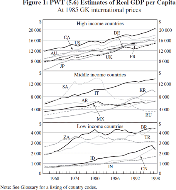
The PWT estimates of real GDP typically result in substantial revisions to exchange rate valuations. Comparing India with the US, for example, the ratio of per capita 1980 GDP is 2.1 per cent at market rates of exchange. The ICP data reveal, however, that non-traded goods and services are much cheaper, relative to traded goods, in India than they are in the US. So the PWT's estimate of real Indian income is much higher, 5.8 per cent of US income.
It is not often appreciated, however, that the PWT approach to comparing inequalities in real income/living standards can be just as problematic as the exchange-rate approach. The problem is that the fixed-price method used for aggregation is subject to substitution bias, as explained by Gerschenkron (1951) and Kravis and Lipsey (1991). PWT analysts have themselves recognised that their measure of purchasing power parity may impart a bias:
The issue arises out of a familiar problem in price and quantity index number construction …Valuation at other than own prices tends to inflate the aggregate value of the bundle of goods because no allowance is made for the substitutions in quantities toward the goods that are relatively cheap…The practical importance of this issue…may loom large in comparisons between countries that have widely divergent price and quantity structures.
(Kravis, Heston and Summers 1982, p 7)
The G-20 group includes countries with widely divergent price and quantity structures, so we can expect the problem of substitution bias in the PWT income comparisons to be substantial. The problem is related to the fact that the ‘international prices’ used in the PWT most closely resemble the price structure of the richer countries[8] and are very different from the price structures that are typically observed in poorer economies. This is partly because the ‘international prices’ are calculated according to a formula that weights the price structure of each ICP country according to its level of GDP – so poorer and less populous countries' economies carry less weight than the large and rich economies of North America and Western Europe. The bias towards developed-economy prices arises also because the countries that have participated in the ICP surveys have not included the world's most populous nation – China.
Given that the GK method measures incomes using the prices of relatively rich countries, we expect that they will overstate the real incomes of poorer countries. This substitution bias can be illustrated by considering expenditures on domestic services and passenger cars for Germany and India – taking the price data from Table 1 and adding in the real quantity data from the 1980 ICP Survey. These data are listed in Table 2.
| Germany | India | India/Germany Per cent | |
|---|---|---|---|
| Local prices (ICP) | |||
| Domestic services | 8.1 DM | 1.1 Rs | na |
| Passenger cars | 1.8 DM | 13.0 Rs | na |
| Real quantities (ICP) | |||
| Domestic services | 6 | 1.7 | 28.3 |
| Passenger cars | 345 | 1.3 | 0.4 |
| Value at German prices (DM) | 656 | 16 | 2.4 |
| Value at Indian prices (Rs) | 4,488 | 19 | 0.4 |
We have already seen that domestic services are relatively cheap in India whilst cars are relatively cheap in Germany. Not surprisingly, per capita consumption of domestic services was relatively high in India, over one-quarter of the German level, whilst their consumption of cars was very low, less than one-half of a per cent of the German level. We can aggregate these expenditures at Indian or German prices to compare national average expenditure on these two items. At German prices, where domestic services are expensive, Indian expenditure looks relatively high – and vice versa. The use of the rich-country prices to value real expenditure ignores the fact that Indian consumers choose to spend relatively more on the services that are cheap in India.
Whilst this example considers expenditures on only two items, the principle of substitution bias, which it illustrates, applies to constant price valuations of GDP as a whole.
Hill (2000) has addressed the problem of measuring substitution bias, adopting two utility-based approaches to establishing bounds on income comparisons. He estimates the parameters of the linear expenditure system, which is derived from the Stone-Geary utility function, to derive utility numbers for each country. He notes the sensitivity of the income ratios to the choice of the reference price vector, illustrated by his finding that the Turkey/US ratio could be as low as 14 per cent or as high as 28 per cent. His other approach is to assume homothetic preferences, implying that income comparisons based on expenditure function ratios are invariant to the reference price vector. This enables him to tighten the bounds on the Turkey/US ratio to the interval between 18 and 25 per cent, leading him to show that the GK measure substantially overvalues the relative income of the poorer country.
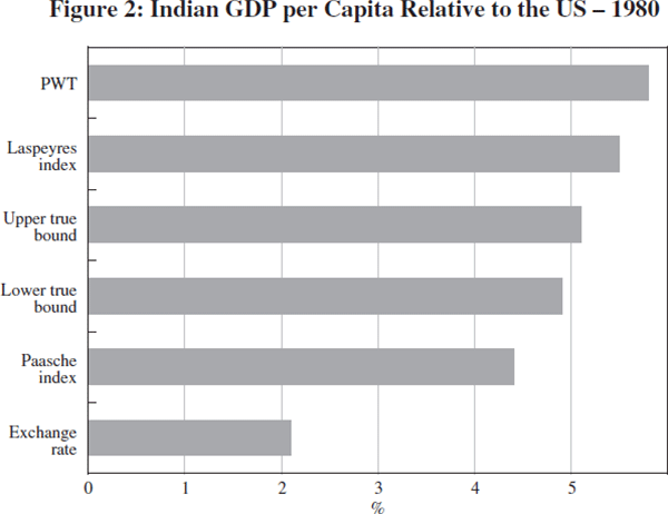
This latter approach is similar to that used by Dowrick and Quiggin (1997). However, whereas Hill examines only bilateral comparisons, Dowrick and Quiggin develop results on the multilateral properties of true index numbers, building on the pioneering work of Afriat (1981). In order to illustrate their method and to highlight the magnitudes of bias involved it is worth explaining results with respect to a particular problem. Using the ICP data set for 1980, what is the value of real income (GDP per capita) in India compared to real income in the US? Exchange rate comparisons give an answer of 2.1 per cent, whilst the Penn World Tables suggest that Indian average income is 5.8 per cent of US income.
These ratios, for Indian income (GDP per capita) relative to the US, are displayed in Figure 2, along with some alternative measures. The Paasche and Laspeyres indices indicate the income ratios which are obtained by evaluating the GDP bundles at US prices or Indian prices respectively. These are intuitively informative indices since they measure the relative values which consumers in either country would put on the consumption bundle of the other. Substitution bias suggests that the Paasche index, using the prices of India to compare the two countries, will understate the true ratio, whilst the Laspeyres, using US prices, will overstate it. This is exactly what we observe: the Laspeyres index is 5.5 per cent, whereas the Paasche Index is 4.4 per cent. If we were concerned only with these two countries it might make sense to choose the geometric mean of the Paasche and Laspeyres ratios, the Fisher ideal index, as our best guess for the true income ratio. There is, however, a well-known problem with the Fisher index: it is intransitive in multi-country comparisons. For example, if we include Brazil in our comparisons, the Fisher index for India/US does not equal the product of the indices for India/Brazil and Brazil/US.
Afriat's solution to this problem can be viewed as a generalisation of the Fisher approach. The attractiveness of the Fisher index is that it is a compromise between the Paasche and Laspeyres indices. But it is the specificity of the Fisher compromise – choosing the geometric mid-point – which makes transitivity impossible. Afriat's solution comes from asking the more general question: is there any set of real income numbers for our 3 (or n) country problem such that the income ratio for each pair of countries lies between the corresponding Paasche and Laspeyres ratios?
If such a set of numbers does exist, the GDP ratios will necessarily satisfy transitivity: for any set of real numbers (a, b, c), a/c = (a/b)*(b/c). Afriat's requirement that the India/Brazil and the Brazil/US ratios lie between rather than at the mid-point of the Paasche and Laspeyres ratios makes it feasible that there may exist such a set of numbers – a ‘true index’ in Afriat's terminology.
The Afriat index is not just a set of convenient numbers. It is a true welfare measure. Afriat (1981) has a remarkable theorem showing that the existence of such a true index, for a given set of observations on prices and quantities, is equivalent to the existence of a common homothetic preference relationship (or utility function) that rationalises the data.[9] That is to say, if there exists a set of Afriat index numbers, then there must also exist some common homothetic utility function such that any country's observed consumption bundle maximises the utility of a representative consumer facing the prices and budget constraint of that country. Moreover, the Afriat index numbers yield bilateral ratios that are the money-metric utility ratios.
In general, if a true index does exist it will not be unique – but we can establish upper and lower bounds to each of the bilateral ratios. These will be tighter than the Paasche-Laspeyres bounds. Using the Afriat method, as described later in this paper, we find that the true utility-consistent India/US income ratio lies between 4.9 per cent and 5.1 per cent.[10] The mid-point of these bounds, a ratio of 5.0 per cent, is the preferred true Afriat income ratio.
Using these true bounds as our benchmark, we can evaluate the degree of bias in different methods of aggregation. Referring to Figure 2 we see that the exchange rate measure lies well below the lower true bound. The exchange rate undervalues India's GDP by more than one-half. We can see that the Penn World Tables correct for the bias inherent in exchange rate valuations of poor countries relative to rich countries; but the substitution bias of the fixed-price method means that the PWT measure has over-valued India's true GDP.
This example illustrates the finding of Dowrick and Quiggin (1997) that neither exchange rate comparisons nor the Penn World Tables comparisons constitute a true index of real incomes. Whilst the exchange rate comparison understates the relative value of incomes in poor countries, the PWT's use of the GK method tends to overstate it.
4. Aggregate PPP Incomes in the G-20 Countries
The 1980 ICP data set was analysed using 128 categories of expenditure for 53 countries satisfying the Afriat-Varian test of common homothetic preferences, implying the existence of true quantity and price indices. The ICP survey covered 60 countries, but only 12 of the current G-20 members were included. Table 3 displays for these 12 countries the various measures of real income (GDP per capita) that we have discussed so far, expressing real incomes as a percentage of US income.
| Aggregation method Per cent | Ratio to true PPP | |||||
|---|---|---|---|---|---|---|
| Exchange rate | GK PPP | True PPP | Exchange rate | GK | ||
| Canada | 93.4 | 101.5 | 91.7 | 1.02 | 1.11 | |
| Germany | 115.8 | 89.1 | 81.2 | 1.43 | 1.10 | |
| France | 105.9 | 85.4 | 77.4 | 1.37 | 1.10 | |
| UK | 81.5 | 72.1 | 61.7 | 1.32 | 1.17 | |
| Italy | 60.6 | 68.0 | 60.9 | 0.99 | 1.12 | |
| Japan | 77.9 | 73.5 | 56.8 | 1.37 | 1.29 | |
| Argentina | 47.7 | 33.6 | 27.7 | 1.72 | 1.21 | |
| Brazil | 18.1 | 29.3 | 27.1 | 0.67 | 1.08 | |
| South Korea | 14.2 | 22.6 | 18.6 | 0.77 | 1.21 | |
| Indonesia | 4.3 | 9.6 | 7.7 | 0.56 | 1.24 | |
| India | 2.1 | 5.8 | 5.0 | 0.43 | 1.16 | |
The same data are displayed in Figure 3. A clear pattern is evident for the least-developed economies: Brazil, South Korea, Indonesia and India. Using the exchange rate to compare incomes with the US, these countries appear very poor. Using the GK method of comparing real incomes, however, has the effect of increasing substantially the relative income estimates. The GK method, taking account of the low prices of non-traded goods and services in these economies, revalues real incomes upwards by more than one-half in the cases of Brazil and South Korea, and more than doubles the estimated real income in the cases of Indonesia and India.
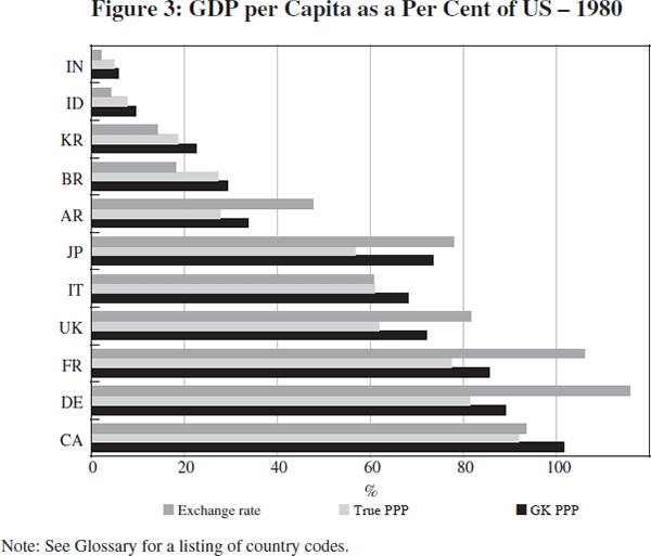
However, the GK method overstates the real income levels of all economies relative to the US. For the poorest economies, the true income measures lie between the foreign exchange and GK estimates.
The most recent ICP survey of national prices was conducted in 1993. Based on the regional data that were released by the World Bank, I have been able to construct a global comparison covering 53 countries. Twelve of the current G-20 member countries participated in this ICP survey. The G-20 participants were not exactly the same as those who had participated in the 1980 survey: Argentina, Brazil and India were replaced by Australia, Turkey and Russia. Table 4 presents a summary of the three different methods of comparing real GDP per capita with that of the US and the results are illustrated in Figure 4.
| Aggregation method Per cent | Ratio to true PPP | |||||
|---|---|---|---|---|---|---|
| Exchange rate | GK PPP | True PPP | Exchange rate | GK | ||
| Japan | 140 | 90 | 84 | 1.65 | 1.07 | |
| Canada | 78 | 82 | 77 | 1.01 | 1.07 | |
| France | 88 | 81 | 75 | 1.18 | 1.08 | |
| Germany | 96 | 78 | 75 | 1.27 | 1.03 | |
| Australia | 68 | 74 | 70 | 0.97 | 1.06 | |
| Italy | 70 | 74 | 70 | 1.00 | 1.05 | |
| UK | 66 | 70 | 66 | 1.01 | 1.07 | |
| South Korea | 31 | 45 | 36 | 0.84 | 1.24 | |
| Turkey | 12 | 26 | 23 | 0.55 | 1.13 | |
| Russia | 11 | 23 | 22 | 0.49 | 1.04 | |
| Indonesia | 3 | 20 | 12 | 0.28 | 1.62 | |
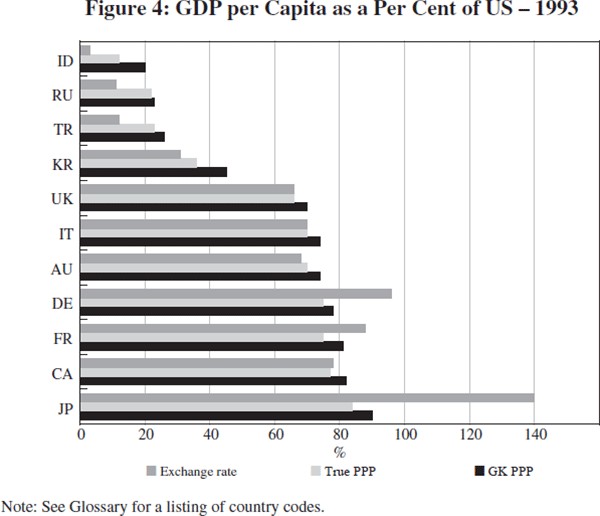
We observe again that the exchange rate comparison understates the relative income level of the poorer economies. Whilst the GK method corrects for the traded-sector bias in the exchange rate comparison, it tends to over-correct – leading to over-valuation of income levels, particularly in the poorest countries.
5. Other Uses of the ICP Data: Analysing Investment Rates
Apart from the aggregate measures of GDP, the ICP data have been widely used in their disaggregated form in order to explain trade patterns and sources of economic growth. For example, the price of investment goods, relative to consumption, is expected to be an important factor in determining the rate of economic growth. The higher the opportunity cost of investment in terms of foregone consumption, the less incentive individuals have to save and invest. Furthermore, a higher price for investment goods implies that a given national savings effort translates into less real investment, hence slower growth. A number of econometric studies, using the ICP data, have found that countries where investment goods are relatively cheap do indeed tend to have higher real investment, thus faster growth.[11]
We can use the ICP disaggregated data in the Penn World Tables to calculate the price of investment relative to consumption for most of the G-20 members. The data are mostly for 1992, but the latest available for Saudi Arabia are 1989. Lacking data for Russia and for unified Germany, I have used the latest available figures for the USSR and West Germany. The data are displayed in Figure 5, with the price of investment/consumption goods on the vertical axis and the level of real GDP per capita on the horizontal axis.
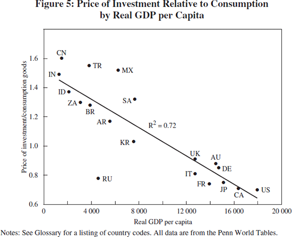
It is apparent that there is a strong negative relationship between the price of investment goods and the level of income – as indicated by the downward-sloping trend line. In the richer OECD countries, many of which are major producers of capital equipment, capital equipment is relatively cheap. On the other hand, in the less-developed economies, the price of capital relative to consumption goods tends to be more than twice as high. In part this reflects the fact that countries without an advanced manufacturing sector have to import much of their capital equipment, incurring transport costs and possibly facing tariff barriers. It also reflects the fact that most consumption goods and services are produced domestically, and that they are relatively cheap in low-wage economies.
These points are illustrated in Figure 6 which again uses PWT data, but this time the price of consumption and the price of investment goods are shown separately. Trend lines for the two series are displayed. It is apparent that although the investment price tends to rise with income, there is a much stronger positive correlation between income and the price of consumption goods. It is this latter relationship which lowers the opportunity cost of investment relative to consumption goods in the richer countries.
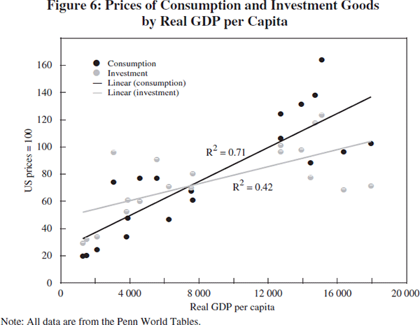
The observation that investment goods tend to be relatively expensive in poorer countries highlights one of the handicaps facing the less-developed economies – they have to sacrifice more of current consumption to achieve a given amount of real investment. This is partly due to the Balassa-Samuelson effect, whereby domestically produced consumption goods are relatively cheap in low-wage economies. But it is also due to the transport costs and, in some cases, tariffs which raise the price of imported capital equipment. Deviations above the trend line in Figure 5 indicate the magnitude of these transport/tariff effects, suggesting the need for policy intervention. Measures to improve transport and communication infrastructure may be needed to reduce transport costs. Consideration may also need to be given to the reduction of import tariffs on capital equipment.
6. Conclusions
The ICP is of increasing importance as policy-makers need to assess the effects of trade and development policies on the growth of their national economies. Without the detailed and standardised measurement of prices and quantities, the core output of the ICP, it is impossible to accurately identify which types of policies and institutional arrangements are most conducive to rising prosperity.
Much attention is devoted to the aggregate measure of real GDP per capita which can be derived from the disaggregated prices and quantities provided by the ICP. I have spent some time in this paper criticising a commonly used method of aggregation, on the grounds that it exaggerates the relative wealth of the poorer economies, and I have suggested that alternative aggregation procedures, including the OECD-preferred EKS method, are preferable for the purpose of assessing relative living standards. This debate should not, in any way, be interpreted as detracting from the value of the ICP. Without the internationally standardised measurement of prices and quantities at the disaggregated level, it is impossible to construct, by any method, economically meaningful aggregates of real income and output. Moreover, the detailed prices and quantities are themselves valuable in terms of assessing microeconomic policies and the impact of trade and exchange-rate policies.
A major limitation of the ICP has been its limited coverage of countries. Outside the OECD, many countries have never participated in the international surveys, whilst others have participated only occasionally. The non-participants miss out on valuable information concerning the comparative price and quantity structure of their own economy, and the global community misses out on additional observations that would help to analyse the efficacy of varied institutions and policies. Where ICP data have not been collected, the authors of the Penn World Tables and organisations such as the World Bank have had to resort to various methods of estimating real (PPP-adjusted) GDP for the non-participating countries. These estimates for the non-benchmark countries are liable to be inaccurate and misleading.
Many issues facing policy-makers today have an important global dimension. The relationship between global warming and the size and growth of global output is of potentially huge significance. The effects of trade and trade policies on living standards, and the distribution of income, are clearly matters of global as well as national concern. It is particularly worrying for estimates of the growth of global output, and changes in global inequality, that the world's most populous country has not been included in any of the ICP surveys to date. Until China is included in these surveys, we are reduced to guestimates of the changes in real output and relative living standards of more than one-fifth of the world's population.
Given their geographic size and diversity, and the evidence of rapid but uneven economic development across regions, it would be desirable for any surveys of countries as large as Russia, India and China to be conducted at the regional level. At the same time, expansion of the ICP surveys into some of the relatively small, but extremely poor, nations of sub-Saharan Africa should reveal important information on the extent to which distortions of the price structures of these countries may be inhibiting their economic development. ICP surveys will not of themselves promote successful and equitable development, but they can provide extremely valuable information for the policy-making process.
Footnotes
EUR213 billion was allocated under the European Regional Development Fund to regions where GDP per capita is less than 75 per cent of the Community average (see <http://www.europa.eu.int/comm/regional_policy/objective1/index_en.htm>). [1]
See Balassa (1964) and Samuelson (1964). [2]
This argument, and the arguments that follow concerning the bias in the Geary-Khamis method of aggregation, are analysed in a formal economic model by Dowrick and Akmal (2002). [3]
Gross domestic product (GDP) is by accounting definition equal to gross domestic income. I use the terms GDP, output and income interchangeably. Gross domestic income differs from national income according to international transfers to non-resident nationals. [4]
The Brazilian currency changed from the cruzeiro to the real in 1994. [5]
In recent years the OECD have used a different aggregation method, the EKS index. The EKS results are often close to the results of the Afriat method, and since they are easier to compute they may be preferred for practical reasons. [6]
The extended PWT data are available at <http://www.worldbank.org/research/growth/GDNdata.htm>, the source used by Melchior, Telle and Wiig (2000). [7]
It is difficult to be precise on this point, because the ‘international prices’ are a weighted average that does not correspond exactly to the price structure of any one country. Nuxoll (1994) suggests that the prices correspond most closely to the prices of Hungary. Dowrick and Quiggin (1997) find the closest correspondence is to the prices of Italy. [8]
This equivalence is explained further by Varian (1982). [9]
We can interpret these numbers as saying that the representative consumer is at least as well off with India's per capita GDP bundle as if they had been offered 4.9 per cent of the US's GDP bundle, whereas the representative consumer is at least as well off with the US bundle as if they had been offered 19.6 times the Indian bundle. [10]
See, for instance, DeLong and Summers (1991), who suggest that it is the price of investment equipment, rather than structures, that matters most and also Sala-i-Martin (1997), who reports a very strong relationship between equipment investment and economic growth. [11]
References
Afriat SN (1981), ‘On the constructability of consistent price indices between several periods simultaneously’, in A Deaton (ed), Essays in the Theory and Measurement of Consumer Behaviour: in honour of Sir Richard Stone, Cambridge University Press, Cambridge, pp 133–161.
Balassa BA (1964), ‘The Purchasing-power Parity Doctrine: A Reappraisal’, Journal of Political Economy, 72(6), pp 584–596.
DeLong JB and LH Summers (1991), ‘Equipment Investment and Economic Growth’, Quarterly Journal of Economics, 106(2), pp 445–502.
Dowrick S and M Akmal (2002), ‘Contradictory Trends in Global Income Inequality: A Tale of Two Biases’, The University of Hong Kong, School of Economics and Finance, Discussion Paper No 355; an earlier version is available at <http://ecocomm.anu.edu.au/economics/staff/dowrick/dowrick.html>.
Dowrick S and J Quiggin (1997), ‘True Measures of GDP and Convergence’, American Economic Review, 87(1), pp 41–64.
Gerschenkron A, assisted by A Erlich (1951), A Dollar Index of Soviet Machinery Output, 1927–28 to 1937, Rand Corporation, Santa Monica.
Hill RJ (2000), ‘Measuring substitution bias in international comparisons based on additive purchasing power parity methods’, European Economic Review, 44(1), pp 145–162.
Kravis IB, AW Heston and R Summers (1982), World Product and Income: International Comparisons of Real Gross Product, Johns Hopkins University Press, Baltimore.
Kravis IB and RE Lipsey (1991), ‘The International Comparison Program: Current Status and Problems’, in P Hooper and JD Richardson (eds), International Economic Transaction: Issues in Measurement and Empirical Research, University of Chicago Press, Chicago, pp 437–468.
Melchior A, K Telle and H Wiig (2000), ‘Globalisation and Inequality: World Income Distribution and Living Standards, 1960–1998’, Royal Norwegian Ministry of Foreign Affairs Studies on Foreign Policy Issues, Report 6B, pp 1–42, available at <http://odin.dep.no/archive/udvedlegg/01/01/rev_016.pdf>.
Nuxoll DA (1994), ‘Differences in Relative Prices and International Differences in Growth Rates’, The American Economic Review, 84(5), pp 1423–1436.
Sala-i-Martin X (1997), ‘I Just Ran Two Million Regressions’, The American Economic Review, Papers and Proceedings, 87(2), pp 178–183.
Samuelson PA (1964), ‘Theoretical Notes on Trade Problems’, Review of Economics and Statistics, 46(2), pp 145–154.
Summers R and AW Heston (1991), ‘The Penn World Table (Mark 5): An Expanded Set of International Comparisons, 1950–1988’, Quarterly Journal of Economics, 106(2), pp 327–368.
Varian HR (1982), ‘The Nonparametric Approach to Demand Analysis’, Econometrica, 50(4), pp 945–973.