RDP 7902: Financial Modelling in Australia Appendix

i) Balance Sheet Restrictions in Models of Integrated Asset Demands^[27]

(a) Equilibrium Models

The agent is assumed to hold a portfolio of n assets, and the demand expressions for each asset are a function of m predetermined variables. Each demand expression is represented by:

In equilibrium models desired asset holdings (A*'s) are assumed to be equal to actual holdings, i.e. = A_r for all r. The complicating factor in these models is that one of the predetermined variables, say x_m, will be identically equal to the sum of the holdings of the other assets, i.e.

This relationship implies that one of the determining factors in an agent's demand for a particular asset will be the total size of the portfolio. (x_m). This variable is commonly known as the constraint variable.

Summing over all demand equations:

Substituting relationship (2):

The restrictions between the parameters which are a result of the balance sheet constraint (2) can be derived by equating like terms in (4), i.e.:

These constraints may be interpreted as:

1. any change in the total value of the portfolio will be spread fully across the asset holdings of the portfolio;
2. any change in other predetermined variables will not affect the total value of asset holdings.

(b) Disequilibrium Models

Brainard and Tobin (1969) argued that the agent may not always be able to achieve his desired asset holdings within one observation period. They suggest the following multiple stock adjustment model.

In section (ii) of this appendix, this model is derived by minimising a quadratic cost function, which measures the cost of being away from desired asset holdings and the costs of adjustment. Expanding (7), using the demand expressions in (1):

Summing over all r equations:

Using the balance sheet constraint (2) and equating like terms, the following restrictions are obtained.

The first two restrictions are equivalent to the equilibrium model, where a change in any exogenous variable apart from wealth, will reshuffle assets but not change the total value of the portfolio, whereas a change in wealth is distributed fully across asset holdings. The third constraint implies that a reshuffling of initial assets will not necessarily change current wealth (x_m).

ii) Multiple Stock Adjustment Models

Consider the quadratic cost function for n assets and m components of expenditure:

A_it: asset holdings; : desired asset holdings

C_it: expenditure components; : desired expenditure

We wish to minimise this quadratic subject to a budget constraint.

where y represents total income (including income from asset holdings). The first order conditions become:

The a_i's measure the cost of being away from the desired position and the b_i's measure the cost of adjustment.

Collecting terms:

Summing over both (6) and (7) and substituting into (8):

But using the result that we can rewrite the L.H.S.:

And, because the desired levels (A^*_it, C^*_it) were derived, subject to the budget identity it is true that:

So that L.H.S. of (9) will simplify to:

Using (9 ) in (12) we obtain an expression for λ:

into

We can now substitute (13),/(6) and (7);

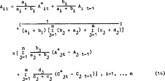
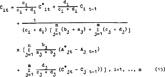
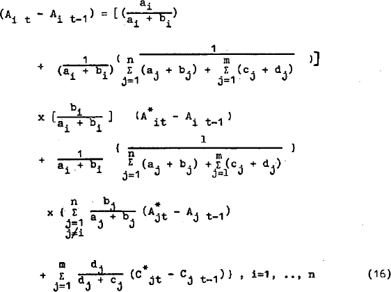
Rearranging (14):

Expression (16) is the multiple stock adjustment model where demand for each asset is affected by the disequilibrium of all the other assets. When the only disequilibrium term which appears in each demand equation is that for the own asset or expenditure component the model is simple stock adjustment.

It is interesting to note that for any asset, j, which has a zero cost of adjustment i.e. b_j = 0, the disequilibrium of this asset will have no effect on the demand equation for any other asset or expenditure component.

Footnote

A more detailed discussion of these restrictions may be found in Purvis (1975). [27]