Figures and Tables | RDP 8809: The Intertemporal Government Budget Constraint and Tests for Bubbles

RDP 8809: The Intertemporal Government Budget Constraint and Tests for Bubbles 8. Figures and Tables

Graham Elliott and Colm Kearney

November 1988

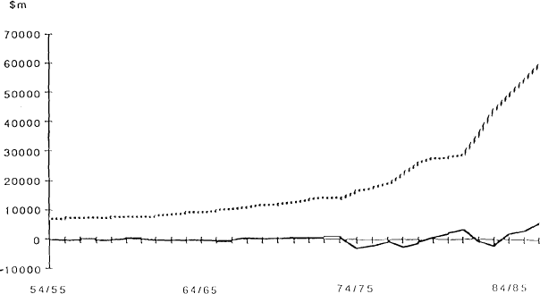
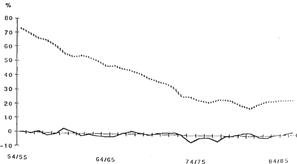
Figure 1 SURPLUS vs DEBT OUTSTANDING

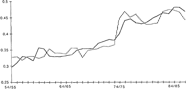
Figure 2 GOVERNMENT SPENDING vs TAXATION PLUS SEIGNIORAGE

TABLE 1: GOVERNMENT DEFICITS AND DEBT OUTSTANDING – 1955 TO 1987
	DEFICIT		DEBT OUTSTANDING
	level	% GDP	level	% GDP
1955	110	1.14	7,007	72.89
1956	159	1.53	7,248	69.59
1957	46	0.41	7,511	66.21
1958	46	0.40	7,475	64.45
1959	271	2.17	7,634	61.25
1960	234	1.70	7,694	55.97
1961	32	0.22	7,871	53.85
1962	358	2.39	8,156	54.49
1963	415	2.56	8,646	53.43
1964	419	2.33	9,188	51.13
1965	183	0.93	9,420	47.65
1966	255	1.23	9,947	47.89
1967	552	2.41	10,394	45.45
1968	643	2.63	10,876	44.55
1969	386	1.40	11,667	42.33
1970	191	0.63	12,015	39.34
1971	10	0.03	12,582	37.29
1972	134	0.36	13,534	35.92
1973	696	1.62	14,133	32.94
1974	281	0.55	13,863	26.99
1975	2,552	4.13	16,494	26.70
1976	3,567	4.90	17,599	24.17
1977	2,685	3.23	19,051	22.91
1978	3,283	3.63	22,531	24.94
1979	3,426	3.35	25,889	25.34
1980	1,989	1.73	27,566	24.02
1981	1,080	0.83	27,856	21.29
1982	553	0.37	28,697	19.40
1983	4,448	2.77	35,504	22.08
1984	7,932	4.40	43,972	24.38
1985	6,720	3.35	49,169	24.51
1986	5,726	2.56	54,783	24.54
1987	2,716	1.10	60,631	24.60
Figures for the Deficit (Commomwealth government only, unadjusted for Public Trading Enterprises and interest payments) and Debt outstanding are from tables 2.14 and 2.23 from Occasional Paper No. 8A published by the RBA. RBA holdings of debt are not included in debt outstanding. Note that this measure of the deficit is that usually considered when fiscal policy is discussed and not the definition of the deficit used in this study.

TABLE 2: TESTS FOR STATIONARITY
	Govt. Exp. Excluding Interest Payments	Govt. Exp. Including Interest Payments	Taxation plus Seignorage
Time Trend t-statistic	2.13	2.29	2.25
DF	−2.38	−2.50	−2.35
ADF	−1.98	−2.00	−1.76
Adjusted DF	−2.26	−2.37	−2.25
Perron and Phillips (PP)	2.36	2.59	2.41
Stock and Watson (SW)	−10.49	−10.93	−10.17
The null hypothesis of non-stationarity is rejected at the 95 per cent significance level if the DF or ADF statistic is greater than −3.60. The critical values for the PP and SW tests (95 per cent) are 7.24 and −21.7, respectively.

TABLE 3: COINTEGRATION TESTS
	Govt Exp Excluding Interest Payments		Govt Exp Including Interest Payments
	Constant	Not Constant	Constant	Not Constant
Constant	0.026 (1.11)	×	−0.023 (−0.91)	×
Alpha	0.934 (15.59)	0.998 (114.27)	0.961 (16.35)	0.908 (118.80)
CRDW	1.26	1.26	1.32	1.19
ADF	−2.34	−3.94	−4.33	−4.41
R2	0.89	0.997	0.90	0.997
	7.36	7.75	9.40	9.77
PP	6.27	6.63	7.94	8.26
SW		−21.56		−20.86
The null hypothesis of no cointegration is rejected at the 95% significance level if the CRDW exceeds 0.386. The critical value for the ADF statistic is −3.37. The Critical value for the SW statistic is −17.5 (95%). The and PP critical values for the cointegrating case are unknown and excluded here as an extra guide.

TABLE 4: TESTS FOR STATIONARITY
Test	Deficit Excluding Interest Payments	Deficit Including Interest Payments
DF	−4.00	−4.27
Adjusted DF	−3.82	−4.16
	7.75	9.13
Perron and Phillips (PP)	6.61	7.71
Stock and Watson (SW)	−21.67	−23.54
The null hypothesis of non-stationarity is accepted at the 95 per cent significance level if the DF statistics are greater than −3.00. The critical values for the and PP tests are 7.24 (95%) and 5.91 (90%) and for the SW test is −14.1 (95%).