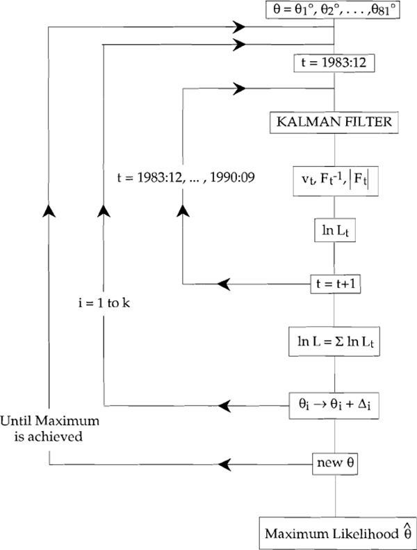
RDP 9111: Monthly Movements in the Australian Dollar and Real Short-Term Interest Differentials: An Application of the Kalman Filter Appendix 2: Our Estimation Procedure – A Flow Chart^[45]

Our estimation process is activated with an initial choice of θ. The Kalman filter recursion begins at our first data observation, December 1983, and uses this first θ to compute the Kalman predictors via:

1. 
2. 

where:

• is the minimum MS linear estimator of the state vector, α_t;
• T is the matrix of coefficients on α_t−1 in the transition equation of our state space model;
• P_t is the error covariance matrix of ;
• Q_t is the covariance matrix for η_t, the vector of disturbance terms in the transition equation.

The following “updating” equations are then applied:

1. 

   where: is known as the Kalman Gain.

   This “correction” term modifies the estimator, ; and .

2. 
3. 

where:

• Z is the vector of coefficients on α_t in the measurement equation;
• F_t is the estimated covariance matrix of the one-step-ahead prediction errors made in estimating the vector of observable explanatory variables and denoted v_t, such that:
  v_t = y_t − E_t−1(y_t).

Therefore, three different errors play a role in the Kalman Filter:

1. , the error in the optimal predictor. This error has covariance matrix P_t.
2. , where is the optimal predictor of α_t given observations up to t−1. E_t−1(P_t) is its covariance matrix.

3. v_t = y_t − E_t−1(y_t), where E_t−1(y_t) is the one-step-ahead prediction of the observation y_t:

   

   F_t is the covariance matrix of v_t.

Given and P_t−1 the workings of the filter can be described by a simple diagram:

The normally distributed prediction errors and their variances generated in this way by the filter are used to calculate the likelihood function. This process is continued for each period in our data set.

The likelihood is then evaluated from the first time period, December 1983. Our search routine, the BHHH algorithm, finds that value of q which maximises log L.

Footnote

This appendix benefits from discussion with Professor Howard Doran of the University of New England, and this diagrammatic representation of the Kalman Filter is an adaptation of that found in Doran (1990). [45]